Organizations and Markets in Emerging Economies ISSN 2029-4581 eISSN 2345-0037
2024, vol. 15, no. 1(30), pp. 165–187 DOI: https://doi.org/10.15388/omee.2024.15.9
Volatility Dynamics of Base Metal Futures: Empirical Evidence from an Emerging Economy
Laxmidhar Samal
P. G. Dept. of Commerce, B.B. (Auto.) Mahavidyalaya, India
laxmidharsamal.bbsr@gmail.com
ORDIC: https://orcid.org/0000-0002-4713-6584
Abstract. The paper examines the leverage effects and the spillover effects in the base metal cash and futures market. The study also attempts to find the trend and the pattern of volatility clustering in the base metal markets of India. Further, the significance of the risk premium and the possible downside risk of the market are also examined. The study confirms that unlike aluminium futures market, leverage effect is found for copper futures traded at MCX, India. Similar to aluminium, it is evident that the market advances generate larger volatility than the market turbulence in the cash and futures market of nickel. The study finds that the variance term (ξ) is not statistically significant for both cash and futures markets, which indicates that the risk premium of the asset is not significant to hedge. Further, unlike copper and aluminium, short-run volatility spillover is absent from the futures to the cash market of nickel. The paper concludes that the long-run volatility shock of futures has a persistent effect on the cash market of aluminium, copper and nickel and vice-versa. Future research might address the cross-volatility spillover between the base metal futures market. Further, the spillover between the Indian and London base metal futures markets is left for future research.
Keywords: futures, volatility, DCC GARCH, base metal, copper, nickel
Received: 15/5/2023. Accepted: 27/2/2024
Copyright © 2024 Laxmidhar Samal. Published by Vilnius University Press. This is an Open Access article distributed under the terms of the Creative Commons Attribution Licence, which permits unrestricted use, distribution, and reproduction in any medium, provided the original author and source are credited.
1. Introduction
After 18 years of lifting the prohibition on the commodity derivative market in India, it has registered all-around significant growth. Various stakeholders participate in futures trading because of its inherent characteristics like hedging, price discovery, price risk management etc. Potential for-profit speculators also participate and provide liquidity to the market (Eswaran & Ramasundaram, 2008). Various futures market participants participate in futures contracts with various objectives, therefore, futures prices depict the expectations of the market (Park & Lim, 2018). Hence, volatility has the main role in hedging, price discovery and selecting an optimal portfolio.
Figure 1
ADT of Base Metal Futures at MCX (RsCrore)
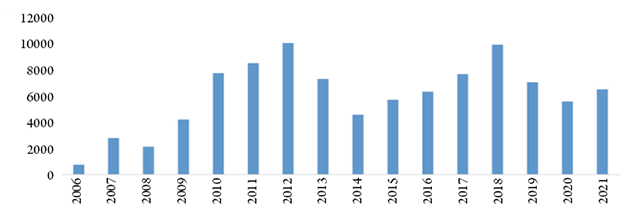
Source: CIYB-2021, MCX, India
The base metal futures market of India registers considerable growth. Figure1 exhibits strong and steady growth in the average daily turnover of the base metal futures. Several reform measures have been undertaken in the recent past, for instance, the domestic benchmark being developed for the base metal, mutual fund houses being allowed to invest in commodity derivatives, trading of commodity futures allowed, etc. (CIYB, 2021). In the year 2013–14, the average daily turnover (ADT) of the base metal futures decreased significantly because of the imposition of commodity transaction tax. After the year 2014–15, there has been consistent growth in the average daily turnover of the base metal futures traded at the MCX platform. Further, due to the COVID pandemic, there was a decrease in the ADT in the year 2019–2020.
Table 1
Annualized Actual Volatility
|
Commodity |
Trading Date |
5 Days |
10 Days |
20 Days |
40 Days |
60 Days |
|
Aluminium |
31st March 2014 |
13.97 |
12.12 |
11.86 |
12.74 |
13.11 |
|
31st March 2015 |
14.64 |
14.46 |
14.32 |
12.25 |
15.01 |
|
|
31st March 2016 |
4.41 |
8.95 |
13.55 |
17.25 |
18.48 |
|
|
31st March 2017 |
9.92 |
7.51 |
9.15 |
13.14 |
14.53 |
|
|
29th March 2018 |
14.16 |
10.84 |
11.46 |
14.99 |
15.74 |
|
|
29th March 2019 |
15.48 |
15.35 |
15.92 |
16.42 |
17.65 |
|
|
31st August 2020 |
4.55 |
10.36 |
12.43 |
12.75 |
12.72 |
|
|
Copper |
Trading Date |
5 Days |
10 Days |
20 Days |
40 Days |
60 Days |
|
31st March 2014 |
14.06 |
14.09 |
16.49 |
15.53 |
14.14 |
|
|
31st March 2015 |
20.71 |
31.47 |
26.28 |
21.61 |
25.79 |
|
|
31st March 2016 |
15.97 |
15.77 |
18.32 |
18.03 |
20.12 |
|
|
31st March 2017 |
13.43 |
15.54 |
14.41 |
20.19 |
21.21 |
|
|
29th March 2018 |
14.23 |
13.60 |
13.30 |
16.85 |
17.24 |
|
|
29th March 2019 |
15.93 |
14.73 |
13.69 |
14.17 |
15.66 |
|
|
31st March 2020 |
13.40 |
41.1 |
31.10 |
23.75 |
21.32 |
|
|
Nickel |
Trading Date |
5 Days |
10 Days |
20 Days |
40 Days |
60 Days |
|
31st March 2014 |
13.29 |
18.37 |
16.32 |
15.47 |
15.32 |
|
|
31st March 2015 |
42.44 |
35.84 |
33.35 |
27.27 |
28.87 |
|
|
31st March 2016 |
21.63 |
25.77 |
40.96 |
39.35 |
36.14 |
|
|
31st March 2017 |
16.16 |
15.80 |
27.35 |
27.97 |
28.76 |
|
|
29th March 2018 |
18.49 |
18.05 |
23.33 |
25.20 |
27.40 |
|
|
29th March 2019 |
17.82 |
17.01 |
22.72 |
24.13 |
23.64 |
|
|
31st March 2020 |
12.02 |
17.35 |
31.41 |
26.24 |
25.70 |
|
|
Lead |
Trading Date |
5 Days |
10 Days |
20 Days |
40 Days |
60 Days |
|
31st March 2014 |
11.80 |
12.92 |
13.55 |
13.14 |
14.41 |
|
|
31st March 2015 |
12.64 |
29.57 |
26.44 |
22.03 |
24.01 |
|
|
31st March 2016 |
20.98 |
20.32 |
20.84 |
24.68 |
24.19 |
|
|
31st March 2017 |
23.26 |
27.26 |
23.26 |
26.55 |
28.74 |
|
|
29th March 2018 |
15.60 |
17.64 |
20.32 |
20.02 |
19.92 |
|
|
29th March 2019 |
14.75 |
15.28 |
18.07 |
18.83 |
17.36 |
|
|
31st August 2020 |
06.12 |
08.03 |
12.17 |
10.99 |
16.63 |
|
|
Zinc |
Trading Date |
5 Days |
10 Days |
20 Days |
40 Days |
60 Days |
|
31st March 2014 |
11.48 |
14.83 |
14.95 |
15.15 |
14.71 |
|
|
31st March 2015 |
11.40 |
16.43 |
15.14 |
14.98 |
17.00 |
|
|
31st March 2016 |
16.90 |
22.33 |
22.07 |
26.62 |
29.71 |
|
|
31st March 2017 |
26.55 |
23.48 |
21.87 |
24.55 |
24.11 |
|
|
29th March 2018 |
11.58 |
15.61 |
20.37 |
20.03 |
19.29 |
|
|
29th March 2019 |
21.22 |
20.47 |
23.07 |
23.15 |
22.09 |
|
|
31st August 2020 |
10.86 |
16.11 |
17.84 |
21.41 |
19.53 |
Source: mcxindia.com
Annualised actual volatility (AAV) indicates the annualised standard deviation of continuously compounded historical returns of the near-month futures contracts of different base metals futures traded at MCX, India. Table 1 presents the 5, 10, 20, 40 and 60 days annualised actual volatility of the different base metals. The near-month futures contracts are considered for the calculation of annualised actual volatility, which is expressed in annualised terms. The annualised actual volatility is computed by using the mathematical notation as follows:
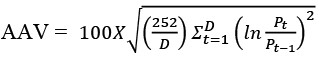
where Pt and Pt–1 refer to the historical closing price of near-month contracts on day t and t–1 and D indicates the number of business days covered for computing historical volatility. The annualised volatility is expressed in percentage terms. The volatility trend of different base metals futures presented in Table 1 indicates that the annualised 5, 10, 20, 40 and 60-day actual volatility of aluminium remains within the range of 12 to 14 percent for the financial year 2014. Unlike in 2014, the annual 60-day actual volatility of aluminium is found higher than other day volatilities for all other financial years. The annualised volatility of aluminium for all financial years remains within the limit of 18.5 percent.
The 5-day annualised actual volatility of copper is the highest in the financial year 2015 and the lowest in the year 2020. Similarly, it is found that the 60-day annualised actual volatility was 28.79 percent in the year 2015 and it was the lowest, i.e., 14.14 percent, for the year 2014. The copper futures market is more volatile than aluminium futures. Except for financial 2014, the 60-day annualised actual volatility of nickel registers more than 23 percent volatility. In the year 2016, the 60-day annualised actual volatility of nickel was the highest, i.e., more than 36 percent. The annualised actual volatility of nickel indicates high volatility in comparison to aluminium futures.
As compared to other commodities, base metals are the backbone of India’s economy as they are used as key inputs for industrial production. Flagship programs of the government of India like Make in India, power for all, housing for all, National Solar Mission, smart city, etc., are directly related to the growth of the base metal industry. The base metal commodities are completely different from other commodities. Unlike agricultural commodities, these are durable and storable. Secondly, in India, the government supports agricultural commodities by paying the minimum support price, but this support is not applied in the case of base metal commodities. Thirdly, the government of India allowed the trading of base metal futures after a long period of allowing agricultural commodities. Importantly, the price of the London Metal Exchange is used as the reference rate for base metal commodities in India. Further, the compulsory delivery specification of base metal futures was introduced in the year 2019–20 in India (Samal & Das, 2023). Unlike other emerging economies, there is no national benchmarking system for the base metals in India. Unlike China and other emerging countries, the base metal market is oligopolistic in India.
The base metal market of India is largely exposed to the international market. Therefore, global factors cause fluctuations in the metal commodities. The value of the asset can fluctuate dramatically because of high volatility and vice-versa. Modelling and forecasting volatility is a significant aspect of financial economics. Nowadays, base metal commodity futures remain a point of attraction for researchers around the globe.
The present study is an attempt to answer the following questions: Does volatility clustering exist in the selected base metal futures market? Are there any leverage effects in the commodity futures market? Which news (good or bad) generates large volatility in the selected base metals markets? Is the risk premium of the market significant to hedge against holding a risky asset? What is the downside potential of the market for the investor? Is there a short-run volatility spillover between cash and futures of base metals traded at MCX, India? Is the long-run spillover effect between the cash and futures market bidirectional?
The present study empirically evaluates the pattern of the volatility of the daily return series of selected base metals cash and futures traded at the Multi Commodity Exchange (MCX) of India. The main characteristics of the series are analyzed by using descriptive statistics. Similarly, the unit root properties of the series are examined by employing ADF and PP unit root tests. The leverage effects are analyzed by employing E-GARCH models, and the news impact curve is studied to answer which news generates larger volatility in the markets of selected base metals. Further, the GARCH-M model is estimated to conclude whether taking a higher risk by holding the base metal futures will lead to higher return for the investor or not. Moreover, the study uses the DCC GARCH model to find the short-run and long-run volatility spillover between the markets of different base metals. Lastly, the VaR model is employed to calculate the downside risk of the markets.
The remainder of the study proceeds as follows. The second part of the paper summarises the existing literature. In the third section, methodology of the study is discussed. The fourth part presents results and discussion, and the last section provides the conclusion, implications and future scope.
2. Review of Literature
There has been extensive study on the commodity futures market considering the volatility of returns, volatility spillover, volatility dynamics, etc. Even though it has been studied extensively both nationally and internationally, very few studies are found on developing nations’ commodity futures markets. A number of papers can be found addressing the volatility of the Indian metals market compared to China and other developing countries.
Locke and Sarkar (1966) studied the volatility dynamics of futures and concluded that in the case of inactive contracts, volatility of returns hurts the market makers. Richter and Sorensen (2002) examined the volatility of returns of soybean futures and options. Their findings confirm that there exists a seasonal pattern of volatility, which is in line with storage theory. By considering 16 agricultural commodities, Chang et al. (2002) extended Richter and Sorensen’s (2002) study and concluded that volatility is persistent in all these agricultural commodities. They used GARCH, EGARCH, and APARCH for analyzing their data. Samal and Das (2022) considered the nickel market and observed higher fluctuation in the cash segment of nickel as compared to futures. Manera et al. (2013) considered both energy and non-energy futures for twenty-six years to examine the effect of speculation on the volatility of returns. They extended the GARCH methodology used by Richter and Sorensen (2002) and concluded that long-run speculation affects negatively impact the volatility of futures return and vice versa. Srinivasan (2012) selected seven commodities and examined whether futures cause cash market volatility or not; the paper concluded that futures are the cause of spot market volatility. In contrast to Srinivasan (2012), Chauhan (2013) observed that the volatility of Chana futures does not influence the volatility of its spot.
Samal and Das (2023) found that the volatility of change in the cash market is higher than the futures market of aluminium traded in India, which contrasts Samal and Das (2022). Sendhil et al. (2013) evaluated the volatility of returns of both spot and futures markets and found that there was persistent volatility in the spot market. Gupta and Varma (2015) studied the flow of volatility between the rubber cash and futures markets and found a bi-directional flow. They found that the volatility of both markets influences each other. By supporting Gupta and Varma (2015), Malhotra and Sharma (2016) also observed bi-directional volatility spillover between the markets of selected commodities. Booth et al. (1997), Zhong et al. (2004), and Fu Qing (2006) studied the different futures markets of different countries, viz., Mexico, China, Norway, etc., and supported the existence of bidirectional spillover. The results of these studies are found in line with the findings of Gupta and Varma (2015) and Malhotra and Sharma (2016).
Many researchers also focused on the maturity effects of the futures market. Anderson (1985) tested the volatility dynamics of agricultural futures and found a maturity effect in commodities like wheat, oat, soybean, and metal futures. Black and Tonks (2000), and Allen and Cruickshank (2000) supported Anderson (1985) and examined Samuelson’s hypothesis. The study observed that the maximum selected contracts support Samuelson’s hypothesis. Floros and Vougas (2006) further extended the study of Black and Tonks (2000), Allen and Cruickshank (2000) and strongly supported Samuelson’s hypothesis. They concluded that ‘volatility depends on time to maturity’.
By examining the Indian commodity futures from 1996 to 2003, Duong and Kalev (2008) found mixed evidence regarding the time-to-maturity effect of volatility. In contrast, Gupta and Rajib (2012) selected eight commodities and concluded that volatility does not depend on time to maturity. Mukherjee and Goswami (2017) examined the volatility of returns of four selected commodities, viz., potato, crude oil, mentha oil, and gold and observed that only near-month gold futures hold Samuelson’s hypothesis. They found persistent volatility for all types of selected contracts.
Bouri et al. (2021) explored the connectedness of realized volatility among the 15 sample commodities from September 2008 to May 2020. The commodities chosen for the study include energy, precious metal, base metal, and agricultural and industrial commodity futures. The research paper concludes that there exists a dynamic cross-commodity connectedness. By extending the study of Bouri et al. (2021), Gong et al.(2021) studied the time varying volatility spillover across the oil and natural gas futures market. The study uses TVP-VAR SV and spillover method proposed by Diebold and Yilmaz (2019, 2012, 2014). The study finds that crude and heating oil are the main net transmitters, whereas gasoline and natural gas are the net receivers of volatility risk information.
Base metal market participants, viz.,producers, consumers, importers, and exporters are highly exposed to market volatility, which arises due to several national and global reasons. Thus, far fewer studies have been conducted concerning the volatility dynamics of the metal futures market of India. Studies presented above have divergent views regarding the volatility dynamics of the commodity futures market. There are some studies which use monthly data for studying volatility, which is inappropriate. Secondly, some studies consider data before 2013, which fails to incorporate the growth of the Indian base metal market. Therefore, by considering base metal commodity futures as financial assets, the present study attempts to examine the volatility clustering effect as well as the leverage effects of selected base metal futures traded at MCX, India. Moreover, the study also examines the short-run as well as the long-run volatility spillover effect between the cash and futures markets. Further, the risk premium of the market, which is significant to hedge against holding a risky asset or not, is investigated.
3. Methodology
The study is based on secondary data which is obtained from the official website of the Multi Commodity Exchange (MCX) of India. Daily closing prices of near-month metal futures are downloaded for a period of 7 years, i.e., from 2013 to 2020. For analysis purposes, we chose three commodities, i.e., aluminium, copper, and nickel out of five base metals traded at MCX, India. The reason for selecting these three base metals is due to their high frequency, continuous trading, and larger volume and value over the period chosen for the study. Before employing any econometric tools, the daily futures price series are converted into their log return form. Thus, the log return price series are calculated as 100×ln (Ft/Ft-1),where Ft refers to the closing prices of futures at day t, and Ft-1 stands for the closing prices of futures at day (t-1).
3.1 Empirical Techniques
Descriptive Statistics. To analyse the basic characteristics of daily return metal futures prices, the study uses descriptive statistics. To test the normality, Jarque-Bera statistics is employed, which implies that:
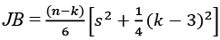 (1)
(1)
Unit Root Test
The study uses the Augmented Dicky-Fuller test (Dicky & Fuller, 1979) as well as the Phillip Perron test (Phillip & Perron, 1988) to investigate the stationarity of the futures return series. The Augmented Dicky-Fuller test can be specified as follows:
Δyt = φ + ∂yt–1 + ∑θΔyt–j + ut (2)
The hypothesis is specified as H0: ∂ = 0, H1: ∂ < 0.
Test for Heteroskedasticity
We perform the ARCH-LM test (Engle, 1982) of heteroskedasticity to investigate the presence of the ARCH effect in the residuals of the return series of base metal futures. To test the ARCH (1) effect, the equation can be modified as:
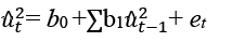 (3)
(3)
The null and alternative hypotheses are specified as H0 : b1 = 0 (homoskedastic), H1: b1 ≠ 0 (heteroskedastic).
E-GARCH Model
The exponential GARCH (E-GARCH) model introduced by Nelson (1991) allows for the testing of asymmetries. The conditional variance of the EGARCH (p, q) model is specified below:
 (4)
(4)
GARCH–M Model
Investors expect a premium in the form of compensation when holding a risky asset. By considering the time-varying risk premium, the model explains the asset return which is written as follows:
Yt = c + ξht + ut (5)
Instead of using variance in Equation 5, if standard deviation is used to capture the risk, then it will be expressed as follows:
 (6)
(6)
Hence, the mentioned model is expressed as:
 (7)
(7)
DCC GARCH Model
The multivariate GARCH model is very useful in studying the interrelations between the time series. Bollerslev (1990) initially introduced the constant conditional correlation GARCH model which was further extended by Jeantheau (1998). The present study uses the DCC GARCH model introduced by Engle (2002) to identify the spillover effect between the spot and futures market of different base metals. Before using the DCC GARCH model, the ARCH effect of variables is tested.
The following bivariate DCC-GARCH (1,1) model is used in this paper:
 (8)
(8)
 (9)
(9)
 (10)
(10)
The parameters α01, α02 represent the average conditional volatility of spot and futures series, respectively; α11, α21are the ARCH parameters, and β11, β21are GARCH parameters which measure sensitivity and persistence. According to Leleng (2014, p.7), ‘the αij∀i, j = 1,2 measures the sensitivity of the shock of the series i on the series j and βi j∀i, j = 1,2 measures the persistence of the shock of the series i on the series j’.
The estimation of the DCC-GARCH model and the likelihood function for  is as follows:
 (11)
(11)
where, θ = (ϕ, ω) are the parameters to be estimated, with:
ϕ = (α0, α1,i , …, αp,i, β1,i, …, βQ,i and (12)
ω = (αDCC, βDCC)
The log-likelihood is defined as follows:
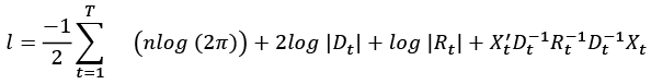 (13)
(13)
The log-likelihood is the sum of a term volatility lv(θ) and another correlation lc (θ, ϕ),
l(θ, ϕ) = lv (θ) + lc(θ, ϕ)
with
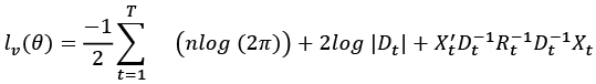
and

According to Leleng (2014, p. 5), ‘the DCC-GARCH model takes into account the change in the relationship between volatility of variables over time and measures the real impact of the volatility of an asset on another asset’.
VaR Model
The risk involved in a particular asset class is essential to measure in a risky environment. Value at risk (VaR) is a widely used technique for the measurement of risk. This piece of research uses parametric VaR to calculate the downside potential of holding the different base metal futures. The VaR models are estimated by using the 95th percentile as well as 99 percentile confidence intervals. The conditional VaR (CVaR) measures the average loss which will be incurred if the VaR is exceeded. By following Rout et al. (2021), at a 99 per cent confidence, the interval parametric VaR is estimated as follows:
VaR = µ – 2.33σ (14)
where µ indicates the mean, and the standard deviation of daily price returns for a period of seven years of the base metal futures contract is represented by σ.
4. Data Analysis and Result Discussion
The movement of daily log returns of three base metals futures is presented in Figures 2, 3 and 4 showing that the movements of returns are different for different periods. Wide swings of the daily log return series of all three base metals indicate that the variance of the return series changes over time. All three series show both wild and calm periods. The wild period refers to the period when large changes are followed by further large changes, whereas the calm period indicates the period when small changes are followed by further small changes. Thus, it implies volatility clustering.
Figure 2
Log Returns Series of Aluminium Futures and Spot Market
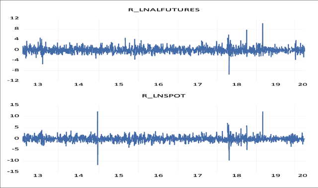
Figure 3
Log Returns Series of Copper Futures and Spot Market
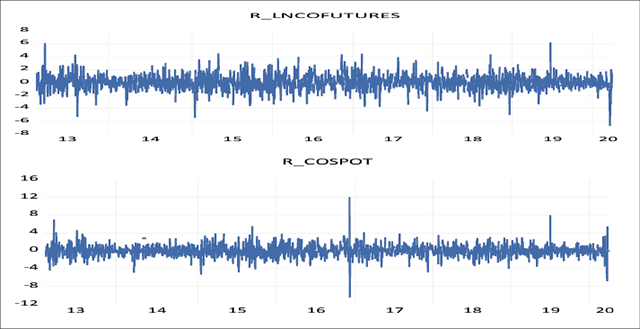
Figure 4
Log Returns Series of Nickel Futures and Spot Market
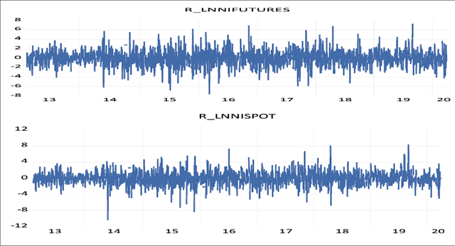
Table 2 presents the summary statistics of the daily log return futures prices of three base metals traded at MCX for the period of seven years, i.e., from 2013 to 2020. The mean daily return of aluminium is positive, in contrast to copper and nickel futures. The median daily returns of all the base metal futures are found to be zero. The maximum daily return of aluminium, copper, and nickel futures is 10.25 percent, 6.14 percent, and 7.26 percent, respectively. Similarly, the minimum daily return of aluminium, copper, and nickel futures was found to be -9.41 percent, -6.67 percent, and -7.58 percent, respectively. Daily returns of nickel futures prices are negatively skewed, unlike daily returns of aluminium and copper futures. The value of kurtosis is higher than 3 for all daily return base metal futures, which indicates that the metal return series is leptokurtic, i.e., fat-tailed. The Jarque-Bera test rejects the null hypothesis of the presence of normality.
Table 2
Descriptive Statistics
|
Descriptive |
Aluminium |
Copper |
Nickel |
|||
|
r_lnalfutures |
r_lnalspot |
r_lncofutures |
r_lncospot |
r_lnnifutures |
r_lnnispot |
|
|
Mean |
0.014 |
0.016 |
-0.004 |
-0.002 |
-0.003 |
-0.000 |
|
Median |
0.000 |
0.000 |
-0.011 |
0.000 |
0.000 |
0.000 |
|
Maximum |
10.254 |
12.250 |
6.135 |
11.990 |
7.260 |
8.334 |
|
Minimum |
-9.410 |
-11.708 |
-6.674 |
-10.416 |
-7.579 |
-10.326 |
|
Std. Dev. |
1.138 |
1.253 |
1.161 |
1.306 |
1.663 |
1.685 |
|
Skewness |
0.640 |
0.631 |
0.0153 |
0.271 |
-0.001 |
-0.063 |
|
Kurtosis |
11.210 |
19.631 |
5.768 |
11.251 |
4.473 |
5.570 |
|
Jarque-Bera |
5314.076 |
21409.94 |
591.189 |
5273.874 |
167.3095 |
510.688 |
|
Probability |
0.000 |
0.000 |
0.000 |
0.000 |
0.000 |
0.000 |
|
Sum |
25.977 |
29.644 |
-7.756 |
-4.936 |
-5.532 |
-0.837 |
|
Sum Sq. Dev. |
2392.936 |
2899.553 |
2495.532 |
3154.921 |
5117.117 |
5258.478 |
|
Observations |
1847 |
1847 |
1851 |
1851 |
1851 |
1851 |
Table 3
Results of Unit Root Test at I (0) (Return Series)
|
Base Metal |
Test |
Variable |
Specifications |
Test Statistics |
Prob. |
|
Aluminium Futures |
Augmented Dickey-Fuller (ADF) |
r_lnalfutures |
Intercept |
-44.775 |
0.000* |
|
Trend & Intercept |
-44.764 |
0.000* |
|||
|
None |
-44.779 |
0.000* |
|||
|
Phillips-Perron (PP) |
r_lnalfutures |
Intercept |
-44.746 |
0.000* |
|
|
Trend & Intercept |
-44.735 |
0.000* |
|||
|
None |
-44.777 |
0.000* |
|||
|
Aluminium Spot |
Augmented Dickey-Fuller (ADF) |
r_lnalspot |
Intercept |
-47.684 |
0.000* |
|
Trend & Intercept |
-47.672 |
0.000* |
|||
|
None |
-47.688 |
0.000* |
|||
|
Phillips-Perron (PP) |
r_lnalspot |
Intercept |
-47.676 |
0.000* |
|
|
Trend & Intercept |
-47.664 |
0.000* |
|||
|
None |
-47.680 |
0.000* |
|||
|
Copper Futures |
Augmented Dickey-Fuller (ADF) |
r_lncofutures |
Intercept |
-43.713 |
0.000* |
|
Trend & Intercept |
-43.701 |
0.000* |
|||
|
None |
-43.723 |
0.000* |
|||
|
Phillips-Perron (PP) |
r_lncofutures |
Intercept |
-43.719 |
0.000* |
|
|
Trend & Intercept |
-43.708 |
0.000* |
|||
|
None |
-43.729 |
0.000* |
|||
|
Base Metal |
Test |
Variable |
Specifications |
Test Statistics |
Prob. |
|
Copper Spot |
Augmented Dickey-Fuller (ADF) |
r_lncospot |
Intercept |
-47.979 |
0.000* |
|
Trend & Intercept |
-47.966 |
0.000* |
|||
|
None |
-47.992 |
0.000* |
|||
|
Phillips-Perron (PP) |
r_lncospot |
Intercept |
-47.986 |
0.000* |
|
|
Trend & Intercept |
-47.973 |
0.000* |
|||
|
None |
-47.999 |
0.000* |
|||
|
Nickel Futures |
Augmented Dickey-Fuller (ADF) |
r_lnnifutures |
Intercept |
-43.977 |
0.000* |
|
Trend & Intercept |
-43.967 |
0.000* |
|||
|
None |
-43.988 |
0.000* |
|||
|
Phillips-Perron (PP) |
r_lnnifutures |
Intercept |
-44.007 |
0.000* |
|
|
Trend & Intercept |
-43.991 |
0.000* |
|||
|
None |
-44.019 |
0.000* |
|||
|
Nickel Spot |
Augmented Dickey-Fuller (ADF) |
r_lnnispot |
Intercept |
-43.791 |
0.000* |
|
Trend & Intercept |
-43.782 |
0.000* |
|||
|
None |
-43.803 |
0.000* |
|||
|
Phillips-Perron (PP) |
r_lnnispot |
Intercept |
-43.814 |
0.000* |
|
|
Trend & Intercept |
-43.806 |
0.000* |
|||
|
None |
-43.826 |
0.000* |
Note.* indicates rejection of null at a 1 per cent significance level.
Before proceeding with the time series modelling, it is inevitable to check the unit root properties of the time series data. The study employs the ADF (Dicky & Fuller, 1979) and the PP test (Phillip & Perron, 1988) to check the unit root properties of the return series of selected base metal futures. The unit root is examined by using three specifications, i.e., intercept, trend, and intercept and none are presented in Table 3. The test statistics and the corresponding probability values of all the selected commodities are significant at the 1 percent level, which rejects the null of presence of unit root. It is evident from Table 3 that the daily log return series of aluminium, copper, and nickel have no unit root at the level for all three specifications. Both tests show the same result.
The study uses the ARCH-LM test (Engle, 1982) of heteroskedasticity to investigate the presence of the ARCH effect in the residuals of daily log return series of base metal futures, which are given in Table 4. After regressing the return series of base metal futures with their lagged return series, we obtained the residuals. Then, to test the ARCH effect, the already obtained residuals are squared off and regressed on their own lags.
The chi-square probability value is zero for aluminium future return series, thus, the null of no ARCH effect in aluminium futures is rejected at a 1 percent level of significance. Similarly, the chi-square probability values for copper and nickel future return series are 0.040 and 0.013, respectively. Therefore, this rejects the null of no ARCH effect at a 5 percent level of significance for copper and nickel futures. As the ARCH-LM statistics are statistically significant for aluminium, copper and nickel futures return series, it confirms the presence of the ARCH effect in residuals of metal series. The spot market of different base metals under consideration also shows similar results.
Table 4
Results of ARCH-LM Test for Residuals
|
Base |
Price |
Hypothesis |
F- Statistics |
Lagrange Multiplier (LM) Test |
Decision |
||
|
Test Result |
Prob. |
Obs*R-squared |
Prob. |
||||
|
Aluminium |
Futures |
H0- There is no ARCH (1) effect in aluminium futures. |
9.927 |
0.000 |
19.673 |
0.000 |
H0 rejected at 1 percent significance level |
|
Spot |
H0- There is no ARCH (1) effect in aluminium spot. |
116.853 |
0.000 |
110.005 |
0.000 |
H0 rejected at 1 percent significance level |
|
|
Copper |
Futures |
H0- There is no ARCH (1) effect in copper futures. |
3.906 |
0.040 |
3.900 |
0.040 |
H0 rejected at 5 percent significance level |
|
Spot |
H0- There is no ARCH (1) effect in copper spot. |
167.230 |
0.000 |
153.512 |
0.000 |
H0 rejected at 1 percent significance level |
|
|
Nickel |
Futures |
H0- There is no ARCH (1) effect in nickel futures. |
6.099 |
0.013 |
6.086 |
0.013 |
H0 rejected at 5 percent significance level |
|
Spot |
H0- There is no ARCH (1) effect in nickel spot. |
9.907 |
0.001 |
9.864 |
0.001 |
H0 rejected at 1 percent significance level |
|
Table 5
E-GARCH Estimation Results
|
Parameters |
Aluminium Futures |
Aluminium Spot |
||||
|
Coefficient |
Test stats. |
P value |
coefficient |
Test stats. |
P value |
|
|
φ |
-0.091 |
-6.329 |
0.000* |
-0.105 |
-8.581 |
0.000* |
|
η |
0.043 |
7.103 |
0.000* |
0.077 |
9.708 |
0.000* |
|
λ |
0.091 |
6.724 |
0.000* |
0.034 |
5.195 |
0.000* |
|
θ |
0.905 |
60.204 |
0.000* |
0.904 |
107.955 |
0.000* |
|
Parameters |
Copper Futures |
Copper Spot |
||||
|
Coefficient |
Test stats. |
P value |
coefficient |
Test stats. |
P value |
|
|
φ |
-0.063 |
-6.488 |
0.000* |
0.084 |
-9.891 |
0.000* |
|
η |
0.009 |
7.027 |
0.000* |
0.055 |
11.754 |
0.000* |
|
λ |
-0.020 |
-2.854 |
0.004** |
-0.009 |
-1.047 |
0.295 |
|
θ |
0.963 |
111.059 |
0.000* |
0.943 |
112.899 |
0.000* |
|
Parameters |
Nickel Futures |
Nickel Spot |
||||
|
Coefficient |
Test stats. |
P value |
coefficient |
Test stats. |
P value |
|
|
φ |
-0.033 |
-4.524 |
0.000* |
-0.039 |
-4.668 |
0.000* |
|
η |
0.057 |
5.682 |
0.000* |
0.073 |
6.585 |
0.000* |
|
λ |
0.021 |
4.388 |
0.000* |
0.022 |
4.715 |
0.000* |
|
θ |
0.900 |
260.143 |
0.000* |
0.905 |
256.159 |
0.000* |
Note. (*) (**) and (***) indicate that parameters are significant at 1, 5 and 10 percent levels, respectively.
The E-GARCH model developed by Nelson (1991) captures the leverage effects of shocks. Table 5 presents the estimated results of the EGARCH model. The shocks in the financial market may arise due to changes in policies, the arrival of new information, the occurrence of incidents, etc. The good and bad news cause market advancements and downfall, respectively. Unlike the standard GARCH model, the E-GARCH model asymmetrically treats the good and bad news.
When (the asymmetric coefficient) λi< 0, it indicates that the negative shocks cause larger volatility than the positive news. Similarly, if λi> 0, it will be concluded that market advances generate larger volatility. The asymmetric effect (λ) is positive and found to be significant at a 1 percent level for both the cash and futures market of aluminium, which implies that market advances generate larger volatility than the market downfall. For the copper futures market, the asymmetric coefficient (λ) is negative and significant at a 5 percent level. It indicates that the negative news generates larger volatility than the good news in the copper futures market. Unlike the copper futures market, the coefficient of the asymmetric term (λ) of nickel cash and futures market is positive and significant at a 1 percent statistical level, which indicates that good news generates larger volatility. The news impact curve of aluminium and nickel cash and futures market shows that the market advances generate larger volatility than the market turbulence.
Figure 5
News Impact Graph of Aluminium Futures
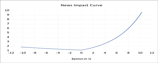
Figure 6
News Impact Graph of Aluminium Spot
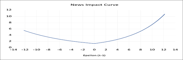
Figure 7
News Impact Graph of Copper Futures
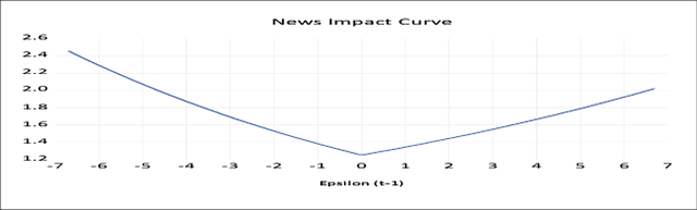
Figure 8
News Impact Graph of Copper Spot
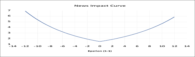
Figure 9
News Impact Graph of Nickel Futures
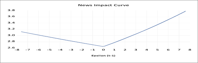
Figure 10
News Impact Graph of Nickel Spot
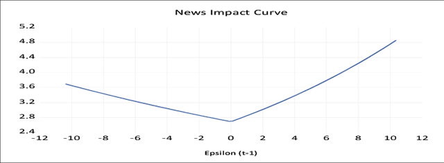
Table 6
GARCH-M Estimation Results
|
Parameters |
Aluminium Futures |
Aluminium Spot |
||||
|
Coeff. |
Test stats. |
P value |
Coeff. |
Test stats. |
P value |
|
|
ξ |
-0.032 |
-0.571 |
0.568 |
-0.088 |
-1.608 |
0.107 |
|
θ |
0.802 |
28.384 |
0.000* |
0.774 |
29.434 |
0.000* |
|
Parameters |
Copper Futures |
Copper Spot |
||||
|
Coeff. |
Test stats. |
P value |
Coeff. |
Test stats. |
P value |
|
|
ξ |
0.064 |
0.669 |
0.503 |
-0.024 |
0.420 |
0.674 |
|
θ |
0.906 |
48.100 |
0.000* |
0.879 |
59.486 |
0.000* |
|
Parameters |
Nickel Futures |
Nickel Spot |
||||
|
Coeff. |
Test stats. |
P value |
Coeff. |
Test stats. |
P value |
|
|
ξ |
-0.079 |
-1.478 |
0.139 |
-0.026 |
-0.574 |
0.565 |
|
θ |
0.962 |
147.554 |
0.000* |
0.950 |
158.973 |
0.000* |
Note. (*) indicates that parameters are statistically significant.
Table 6 presents the estimated results of the GARCH-M model. The GARCH-M model allows the conditional mean to depend upon its own conditional variance. The model considers the time-varying risk premium to explain the asset return. The results indicate that the coefficients in the mean equation (ξ) for aluminium spot and futures are negative and not significant. This implies that taking a higher risk by holding the aluminium futures will not lead to higher returns for the investor. In other words, the risk premium is not significant to hedge against holding a risky asset. A similar result is found for the copper and nickel market.
From the results in Table 7, it is observed that the coefficients of the ARCH effect (α1) are significant for all commodities. Similarly, the coefficients of the GARCH term (β1) stand significant at a 1 percent statistical level. As the GARCH coefficient is considerably greater than the ARCH coefficient, it indicates that the volatility of base metal contracts is more sensitive towards their lagged values over the period chosen for the study. This is observed for all the base metal futures contracts. The coefficient of the short-run volatility spillover (dccα1) is significant for copper at a 1 percent statistical level, which indicates there is a short-run volatility spillover from the futures to the cash market of copper.
Table 7
DCC GARCH (1, 1) Estimation Results (Spillover Effect from Futures to Spot Market)
|
Parameters |
Aluminium |
Copper |
Nickel |
||||||
|
Coeff. |
t- stats. |
p-value |
Coeff. |
t- stats. |
p-value |
Coeff. |
t- stats. |
p-value |
|
|
Ω |
0.000 |
2.557 |
0.010* |
0.000 |
21.107 |
0.000* |
0.000 |
3.860 |
0.000* |
|
α1 |
0.133 |
2.528 |
0.011** |
0.025 |
28.786 |
0.000* |
0.035 |
11.025 |
0.000* |
|
β1 |
0.709 |
7.749 |
0.000* |
0.943 |
85.011 |
0.000* |
0.947 |
187.401 |
0.000* |
|
dccα1 |
0.033 |
1.698 |
0.089*** |
0.066 |
5.272 |
0.000* |
0.044 |
0.031 |
0.163 |
|
dccβ1 |
0.934 |
16.769 |
0.000* |
0.923 |
57.244 |
0.000* |
0.810 |
2.651 |
0.008* |
Note. (*) (**) and (***) indicate that parameters are significant at 1, 5 and 10 percent levels, respectively.
Similarly, it is found that there exists a short-run volatility spillover from futures to cash market of aluminium as the coefficient of short-run volatility is found significant at a 10 percent level. Unlike copper and aluminium, there is no short-run volatility spillover from the futures market to the cash market of nickel traded at MCX, India. The coefficient of the long-run spillover effect (dccβ1) is found significant at a 1 percent level for all the three base metals, which indicates there exists long-run volatility spillover from futures to cash market of aluminium, copper and nickel. The results of the model are consistent with the theory that the coefficients of short-run and long-run spillover are found less than one for all the three commodities, i.e. (dccα1 + dccβ1< 1).
Table 8
DCC GARCH (1, 1) Estimation Results (Spillover Effect from Spot to Futures Market)
|
Parameters |
Aluminium |
Copper |
Nickel |
||||||
|
Coeff. |
t- stats. |
p-value |
Coeff. |
t- stats. |
p-value |
Coeff. |
t- stats. |
p-value |
|
|
Ω |
0.000 |
2.192 |
0.028** |
0.000 |
1.831 |
0.040* |
0.000 |
10.522 |
0.000* |
|
α1 |
0.112 |
3.189 |
0.001* |
0.079 |
1.901 |
0.037** |
0.054 |
13.731 |
0.000* |
|
β1 |
0.672 |
6.592 |
0.000* |
0.824 |
8.907 |
0.000* |
0.915 |
128.051 |
0.000* |
|
dccα1 |
0.033 |
1.700 |
0.088*** |
0.066 |
5.272 |
0.000* |
0.044 |
1.369 |
0.171 |
|
dccβ1 |
0.935 |
16.788 |
0.000* |
0.923 |
57.250 |
0.000* |
0.810 |
2.596 |
0.009* |
Note. (*) (**) and (***) indicate that parameters are significant at 1 percent, 5 percent and 10 percent levels, respectively.
By considering the results of Table 8, the study confirms the existence of short- run and long-run volatility spillover from the spot to the futures market of copper as both the parameters of volatility spillover are found significant at a 1 percent statistical level. Similarly, volatility spillover is observed from the cash to the futures market of aluminium. Unlike copper and aluminium, the study confirms no short-run volatility spillover from the spot to the futures market of nickel. However, long-run volatility spillover is observed from nickel cash to futures market.
The long-run volatility shock of futures has a persistent effect on the cash market of aluminium, copper and nickel, and vice-versa. The study confirms that there is bidirectional long-run volatility spillover between the cash and futures market of different base metals traded at MCX, India. Similarly, unlike nickel short-run volatility, spillover is observed between the spot and futures markets of copper and aluminium.
Table 9
Parametric Value at Risk (VaR) and CVaR: Spot Returns
|
Commodities |
Observations |
VaR |
VaR |
CVaR |
CVaR |
Rank |
Rank |
|
Aluminium |
1847 |
-2.044 |
-2.899 |
-2.568 |
-3.324 |
1 |
1 |
|
Copper |
1851 |
-2.151 |
-3.041 |
-2.696 |
-3.483 |
2 |
2 |
|
Nickel |
1851 |
-2.774 |
-3.922 |
-3.478 |
-4.494 |
4 |
4 |
Table 10
Parametric Value at Risk (VaR) and CVaR: Futures Returns
|
Commodities |
Observations |
VaR |
VaR |
CVaR |
CVaR |
Rank |
Rank |
|
Aluminium |
1847 |
-1.858 |
-2.634 |
-2.334 |
-3.020 |
1 |
1 |
|
Copper |
1851 |
-1.914 |
-2.706 |
-2.399 |
-3.099 |
2 |
2 |
|
Nickel |
1851 |
-2.738 |
-3.872 |
-3.433 |
-4.435 |
5 |
5 |
The results of value at risk (VaR) indicate the likelihood of occurring of a specific loss on a certain confidence interval. The downside risk has always remained an important aspect of the risk assessment system. Tables 9 and 10 present the estimated results of VaR and CVaR, respectively. The number of data points considered for measuring the downside risk is mentioned under the observations column. Nickel is more prone to downside risk than aluminium and copper, which have a lesser downside risk. The maximum loss the investor can incur by holding an aluminium futures contract is -2.63 percent at a 99 percent confidence interval. This percentage is a little higher, i.e. -2.71% for copper futures series. Among the base metal futures, return series of nickel has the highest downside risk.
5. Conclusion
Volatility analysis plays a key role in making any financial decision. Volatility measures the amplification of the variation in the price of a time series variable. The majority of the studies opined that the past volatility of the financial time series influences the present volatility. Moreover, studies have also observed leverage effects, i.e., the market downturn generates larger volatility than the same magnitude of market advances (Leleng,2014). Volatility is a source of both risk and opportunity, therefore the analysis of the volatility of a financial asset is a source of interest for policymakers, researchers and investors.
Wide swings of the daily log return series of all three base metals indicate that the variance of the return series changes over time. The return series of all selected metals are leptokurtic, i.e., fat-tailed. The study finds that the daily log return series of aluminum, copper, and nickel have no unit root at the level for all three specifications. This is confirmed by both the ADF as well as the PP unit root tests. The cash and futures series of different base metals under consideration confirm the presence of the ARCH effect in residuals at a statistically significant level. Unlike aluminium futures, market leverage effect is found for copper futures traded at MCX, India. For the copper futures market, the asymmetric coefficient (λ) is negative and significant at a 5 % level. It indicates that the market turbulence generates larger volatility than the market advances in the copper futures market. Similar to aluminium, the cash and futures market of nickel shows that the market advances generate larger volatility than the market turbulence. The study also observes that the variance term (ξ) is not statistically significant for both cash and futures markets, which indicates that the risk premium of the asset is not significant to hedge.
Unlike copper and aluminium, there is no short-run volatility spillover from the futures market to the cash market of nickel traded at MCX, India. The coefficient of the long-run spillover effect (dccβ1) is found statistically significant for all the three base metals, which indicates there exists long-run volatility spillover from futures to cash market of aluminium, copper and nickel. The long-run volatility shock of futures has a persistent effect on the cash market of aluminium, copper and nickel and vice-versa. The study confirms that there is a bidirectional long-run volatility spillover between the cash and futures market of different base metals traded at MCX, India. The maximum loss the investor can incur by holding an aluminium futures contract is -2.63 % at a 99 percent confidence interval. Among the base metal futures, return series of nickel has the highest downside risk.
Unlike agricultural commodities, base metals are used as an important input for producing industrial products, and their prices are influenced by global factors. Secondly, unlike agricultural produce, there is no minimum support price announced by the Government. The Indian base metal market is exposed to price swings in the international market as the London Metal Exchange Price is used as a reference price all over the world. Further, a large segment of the metal market consists of small and marginal sections which do not have the technical expertise and operate with financial constraints thereby not being able to participate in the futures market.
6. Implication and Future Scope
The study will help the investors to assess the potential risk of the market. By using the results, the market participant will be able to frame different trading strategies. The potential investors will be able to assess the downside risk of the market. The results of the leverage effect will help the speculators and arbitragers in designing their trading strategies. This piece of research will help the regulating agencies frame policies for further deepening the futures market.
The study considers only three base metal futures contracts which can be increased by the future course of research. The study period chosen is seven years only, therefore it can be extended by future research. Moreover, the future scope of research could address the cross-volatility spillover between the different base metal futures markets. Further, the spillover between the Indian and London base metal futures markets is left for the future course of research.
References
Allen, D.E., & Cruickshank, S.N. (2000). Empirical Testing of the Samuelson Hypothesis: An Application to Futures Market of Australia, Singapore and UK.(Working Paper).School of Finance and Business Economics, Edith Cowan University.
Anderson, R.W. (1985). Some Determinants of Volatility of Futures Prices. Journal of Futures Market, 5(3), 331–348.
Asteriou, D.,& Hall, S.G. (2007). Applied Econometrics: A Modern Approach. Palgrave Macmillan.
Black, J.,& Tonks, I. (2000). Time series volatility of commodity futures prices. Journal of Futures Market, 20(2), 127–144.
Bollerslev, T. (1986). Generalized autoregressive conditional heteroskedasticity. Journal of Econometrics, 31(3), 307–327.
Booth, G.G., Martikeinan, T.,& Tse, Y. (1997). Price and volatility spillover in the Scandinavian stock market. Journal of Banking and Finance, 2(6), 811–823.
Chang, C., MCAleer, M.,& Tansuchat, R. (2012). Modelling Long Memory Volatility in Agricultural Commodity Futures Returns(Working Paper). Complutense University of Madrid.
Chauhan, K.A., Singh, S.,& Arora, A. (2013). Market Efficiency and Volatility Spillover in Futures and Spot Commodity Market: The Agricultural Sector Perspective. SBIM,6(2), 61–84.
Dickey, D.A.,& Fuller, W.A. (1979). Distribution of the Estimators for Autoregressive Time Series with a Unit Root. Journal of the American Statistical Association, 74, 427–431.
Duong, N.H.,& Kalev, S.P. (2008). The Samuelson’s hypothesis in the futures market: An analysis using futures data. Journal of Banking Finance, 32(4), 489–500.
Easwaran, R.S.,& Ramasundaram, P. (2008). Whether Commodity Futures Market in Agriculture is Efficient in Price dDscovery? – An Econometric Analysis. Agricultural Economics Research Review, 21, 337–344.
Engle, R. F. (1982). Autoregressive Conditional Heteroskedasticity with Estimates of the Variance of the of UK Inflation. Econometrica, 50(4), 987–1007.
Floros, C., & Vougas, V.D. (2006). Samuelson’s hypothesis in Greek stock index futures market. Investment Management and Financial Innovations, 3(2), 154–170.
Fu, L.Q.,& Qing, Z.J. (2006). Price Discovery and Volatility Spillover: Evidence from Chinese Spot-Futures Market. China and World Economy, 14(2), 79–92.
5Gong, X., Liu, Y., & Wang, X. (2021). Dynamic volatility spillovers across oil and natural gas futures markets based on a time-varying spillover method. International Review of Financial Analysis, 76(2021), 1–14.https://doi.org/10.1016/j.irfa.2021.101790.
Gujurati, D.N. (1995). Basic Econometrics.McGraw-Hill, Singapore.
Gupta, A., & Varma, P. (2015). Impact of Futures Trading on Spot Markets: An Empirical Analysis of Rubber in India. East Economic Journal, 42(3), 1–14.
Gupta, K.S.,& Rajib, P. (2012). Samuelson’s Hypothesis and Indian Commodity Derivative Market. Asia Pacific Financial Markets, 19, 331–352.
Leleng, K. (2014). What [does] DCC GARCH model tell us about the effect of the gold price’s volatility on the South African exchange rate? Munich Personal RePEc Archive, 72584.
Locke, P., & Sarkar, A. (1996). Volatility and Liquidity in Futures Markets. (Research Paper 9612). Federal Reserve Bank of New York.
Malhotra, M.,& Sharma, K.D. (2016). Volatility Dynamics in Oil and Oils Seed Spot andFutures Market of India. Vikalpa: The Journal for Decision Makers, 41(2), 132–148.
Manera, M., Nicoloni, M., & Vignati, I. (2013). Futures price volatility in commodities market: The role of short term vs. long term speculation (DEM Working Paper Series 42). University di Pavia.
Mukherjee, I.,& Goswami, B. (2017). The volatility of returns from commodity futures: Evidence from India. Financial Innovation, 3(15), 1–23.
Multi-Commodity Exchange of India (2019). Commodity Insight Year Book 2019. MCX, Mumbai, India.
Multi-Commodity Exchange of India (2020). Commodity Insight Year Book 2020. MCX, Mumbai, India.
Nelson, D.B. (1991). Conditional Heteroskedasticity in Asset Returns: A New Approach. Econometrica, 59(2), 347–370.
Park, J.,& Lim, B. (2018). Testing Efficiency of London Metal Exchange: New Evidence. International Journal of Financial Studies, 6(32), 1–10.
Philips, P.C.B.,& Perron, P. (1988). Testing for a unit root in time series regression. Biometrica, 75(2), 335–346.
Rajip, P. (2014). Commodity Derivative and Risk Management. PHI Learning Private Ltd, Delhi.
Rana, S.B. (2020). Dynamics of Time Varying Volatility in Stock Returns: Evidence from Nepal Stock Exchange. Journal of Business and Social Science Research, 5(1), 15–34.
Richter, M., & Sorensen, C. (2002). Stochastic Volatility and Seasonally in Commodity Futures and Options: The Case of Soybean (Working Paper). Copenhagen business school.
Rout, B.S., Das, N.M., & Rao, K.C. (2021). Competence and efficacy of commodity futures market: Dissection of price discovery, volatility, and hedging. IIMB Management Review,33(2), 146–155. https://doi.org/10.1016/j.iimb.2021.03.014.
Samal, L.,& Das, S.K. (2023). Hedging Effectiveness and Influential Direction between Spot and Futures Market of Aluminium: An Evidence from India. Business Perspectives and Research. https://doi.org/10.1177/22785337221148537
Samal, L., & Das, S.K. (2022). Price Synergy in Spot and Future Market: A Study on Nickel Trade at MCX, India. Orissa Journal of Commerce. 43(4), 46–58.DOI: https://doi.org/10.54063/ojc.2022.v43i04.04
Securities and Exchange Board of India (2018). Handbook of Statistics on the Indian Securities Market 2017. SEBI, Mumbai India.
Securities and Exchange Board of India (2019). Handbook of Statistics on the Indian Securities Market 2018. SEBI, Mumbai India.
Sendhi, R., Kar, A., Mathur, C.V.,& Jha, K.G. (2013). Price Discovery, Transmission and Volatility: Agricultural Commodity Futures. Agricultural Economic Research Review, 26(1), 41–54.
Srinivasan, P. (2011). Price Discovery and Volatility Spillover in Indian Spot Futures Commodity Market. The UPI Journal of Behavioral Finance, 9(1), 70–85.
Swain, A., & Samal, L. (2017). Hedging Efficiency of Futures Market on Cash Crops (Jute) – An Indian Experience. International Journal of Advanced Research, 5(2), 1725–1742. http://dx.doi.org/10.21474/IJAR01/3335
Zhong, M., Darrat, A.F., & Otero, R. (2004). Price discovery and volatility spillover in index futures market: Some evidence from Mexico. Journal of Banking and Finance, 28(12), 3037–3054.