Organizations and Markets in Emerging Economies ISSN 2029-4581 eISSN 2345-0037
2022, vol. 13, no. 2(26), pp. 467–489 DOI: https://doi.org/10.15388/omee.2022.13.89

Investigation of Fractal Market Hypothesis in Emerging Markets: Evidence from the MINT Stock Markets

Yunus Karaömer
Hatay Mustafa Kemal University, Turkey
yk.karaomer88@gmail.com
https://orcid.org/0000-0002-6377-1326

Abstract. This study aims to investigate the market efficiency of emerging stock markets, namely the Mexico, Indonesia, Nigeria, and Turkey (MINT) stock markets based on the Fractal Market Hypothesis. For this purpose, the ARFIMA and ARFIMA-FIGARCH type models are used to analyze the MINT stock return series. In this study, the dataset encompasses the daily frequency data of the MINT stock market indices from January 12, 2018, to January 12, 2022. The empirical findings show that long memory is reported for the MINT stock returns. The long memory in the returns implies that the MINT stock prices follow a predictable behavior that is consistent with the Fractal Market Hypothesis. The long memory in the volatility implies that the uncertainty or risk is an important factor in the formation of price movements in the MINT stock prices. Moreover, the MINT stock prices consist of the effect of shocks and news that occurred in the recent past. Thus, this study contributes to investors, academics, and market regulatory authorities. Besides, as far as we know, the current literature on the analysis of the fractal market hypothesis to explore the efficiency of the MINT stock markets has not been found.

Keywords: long memory, fractal market hypothesis, emerging markets

Received: 14/4/2022. Accepted: 7/11/2022
Copyright © 2022 Yunus Karaömer. Published by Vilnius University Press. This is an Open Access article distributed under the terms of the Creative Commons Attribution Licence, which permits unrestricted use, distribution, and reproduction in any medium, provided the original author and source are credited.

1. Introduction

Market efficiency is one of the important concepts widely researched in neoclassical finance. The Efficient Market Hypothesis (EMH) is based on the original contributions from Bachelier (1900), Cowles (1933), Kendall (1953), Samuelson (1965), and Fama (1965). These authors claim that in an information efficient market, price changes cannot be predicted if the prices of stock reflect all the expectations of the investors and all the available information in the market. More specifically, Fama (1970) defines the efficiency of a market as the one in which the stock prices always fully reflect all the information available in the market. According to the hypothesis, there is a correlation between stock prices and information because the stock prices are always formed according to the new information announced. In the EMH, markets scale from an asymmetric information environment to a symmetric information environment. Thus, there is no asymmetric information problem in the EMH, and the prices in the market are formed randomly. In other words, the variations in prices follow a normal distribution (Panas & Ninni, 2010). However, in literature, many studies find that financial time series do not exhibit random walks as assumed by the EMH, and the price variations do not follow the normal distribution. Bam et al. (2018) investigated the random walk of the stock prices of the Nepalese Commercial Banks, and found that the stock prices of the Nepalese Commercial Banks are not a random walk process. Rehman et al. (2018) examined the random walk of the stock prices of the KSE 100 index, S&P BSE 500 index, and CSE All Share index. They found that the stock price does not follow a random walk. Sadat and Hasan (2019) investigated the random walk of the Dhaka stock exchange indices and found that prices of the Dhaka stock exchange index do not follow a random walk.

Mandelbrot (1963) introduced the fractal model to describe a particular class of objects that exhibit complex behavior. He drew attention to the self-similarity feature of cotton prices and commodity prices and included the concepts of fractal, self-similarity, fat tails in the return distribution, and long-term memory in financial modeling. The word fractal is derived from the word fractus, which means broken or shattered. Fractals exhibit self-similarity; parts of an object show similar structural features as the whole repeating itself. Fractals also exhibit a property called scale invariance, where the same or similar pattern is repeated across multiple dimensions or time scales. A set that is self-similar and repeats the same patterns at every scale is usually called a fractal (Erokhin & Roshka, 2018). The concept of a fractal is illustrated by the fact that each scale is similar to, but not identical to, other scales, as seen in the sampling of individual branches of a tree qualitatively similar to other branches, but each branch is unique. Fractal analysis has the feature of distinguishing fractals from other time series by revealing a self-similar statistical structure (Tebyaniyan et al., 2020). The Fractal Market Hypothesis (FMH) is a consequence of stating that a financial time series looks the same on different time scales, at least in a statistical sense; for example, the distribution of price values within a day is similar to the distribution of one day, the month is similar to the distribution for a year and so on (assuming there is enough data at each time scale to make the distribution— the calculated histogram— statistically significant) (Blackledge & Lamphiere, 2021). The principle of self-similarity is explained by the concepts of long-term memory or long-term dependence in the financial time series. The existence of long-term memory is compatible with the proposed fractional Brownian motion model. It was certainly Mandelbrot who proposed the use of the fractional Brownian model of motion in economics in the early 1960s (Arouxet et al., 2022). The report published by Hurst (1951) guided Mandelbrot on how to model the long-term dependence effect. Hurst is a hydrologist who started work on the Nile River Dam project in 1907 and stayed in the Nile region for 40 years. He worked at the dam to control the water. In this report, Hurst examined the strong dependence between natural events, such as river flow, times of drought, and extension of floods from one year to the next, using the Hurst exponent. Fractional Brownian motion, which is the new model developed by Mandelbrot, is described by an equation including the Hurst exponent (Graves et al., 2017). The Hurst exponent is widely used as a method to measure long-term memory properties. This measure quantifies the degree of persistence of similar price change patterns and is closely related to the weak-formed EMH (Eom et al., 2008).

Peters (1994) expanded the fractal model developed by Mandelbrot (1963) and proposed the FMH as an alternative theory to the EMH by combining fractals, chaos theory concepts, and traditional quantitative methods. The FMH emerges with the understanding of self-similarity in financial time series. The FMH is based on two key components, market liquidity, and information. Market liquidity arises as a result of investors buying and selling transactions. For market liquidity, investors must have different views on the value of a security. This difference may arise for two reasons. Firstly, one investor has information on the value of the security, while the other investor does not or cannot access the information. Second, two investors not only access information simultaneously but also give different weights to information during different time periods in which they invest. Investors are not rational investors, they are heterogeneous, consisting of long-term and short-term investors. The FMH, unlike the EMH, is complex and constantly evolving (Güler, 2019). The five key assumptions of the FMH can be summarized as follows (Brătian et al., 2021): (a) the financial market is stable if investors cover a wide variety of investment horizons; (b) the information set is influenced by short-term factors and market sentiment dominated by fundamentals in the long term; (c) long-term investors will trade short-term information if a market event casts doubt on the fundamentals; (d) prices reflect a combination of technical and fundamental analysis; (e) financial security is not related to the economic cycle; it will not be a long-term trend.

Comparing the EMH and FMH, the EMH regards the market as a linear and isolated system. The price returns are normally distributed. The market has a single equilibrium and is always in equilibrium with deviations that are highly infrequent and negligible deviations. The past events have no effect on future prices, as the market behaves randomly. For this reason, the price returns indicate a short memory property. By contrast, the FMH regards the market as a non-linear and open system. The price returns are not normally distributed and indicate the fat tails and high peaks. There are different equilibria for each investment horizon, so the market cannot reach a single equilibrium. Due to the self-similarity in fractal structures, past events have an effect on future prices. For this reason, the price returns indicate a long memory property (Sarpong, 2017; Liu et al. 2020).

Recently, different economic classifications such as the MENA countries, the BRICS countries, and the MINT countries have come to the fore as well as the concepts of developed countries, emerging countries, and developing countries. The MINT countries are the next four largest emerging markets; the term was coined in 2012 by Jim O’Neill. These countries are generally emerging economies with similar characteristics. First, they have a large and growing population with suitable demographics. Second, these countries are geographically placed in an advantageous position (Adebayo et al., 2020). While making such classifications, the macroeconomic similarities of the countries are considered, which helps international investors to diversify by choosing countries with low correlation degrees while making portfolio investments, thus reducing risk. For this reason, in this study, a long memory property in stock return and volatility of MINT was investigated with ARFIMA and ARFIMA-FIGARCH type models to open a new horizon for investors. The speed with which each new information coming to the market reaches the price and the extent to which it is reflected on the market may differ according to the developed and emerging markets. Investors in emerging markets may react slowly and late to new information, since each new information that comes to the market reaches emerging markets at a slow rate, unlike developed markets. In emerging markets, many reasons with economic, political, and social content can cause volatility of different sizes in prices. For this reason, studying the long memory behavior in the MINT stock returns based on the FMH may be important for investors, portfolio managers, financial institutions, portfolio diversification, portfolio optimization, risk management, hedging, price discovery, and investment decisions. In addition, emerging countries like MINT need both domestic and foreign capital investments for economic growth. Investors who trust that the market is efficient would be more willing to invest in these markets, and the cost of capital in these countries would decrease. Thus, this study contributes to investors, academics, and market regulatory authorities. Besides, as far as we know, the current literature on the analysis of fractal (as defined by the fractal market hypothesis) to explore the efficiency of the MINT stock markets has not been found.

The rest of this study is organized as follows: Section 2 presents a review of the relevant literature. Section 3 explains the methodology. Section 4 describes the data and preliminary statistics. Empirical findings are discussed in Section 5. Finally, Section 6 provides the conclusion.

2. Literature Review

Financial market behaviors can be characterized as complex systems. From this point of view, the financial market behaviors can be explained with a fractal structure property. The fractal structure properties can provide important insights into the long-term memory of market behavior because the parts are all similar (Aygören, 2008). The principle of self-similarity is explained by the concepts of long-term memory or long-term dependence in the financial time series. In a stationary time series, the term “long-term memory” or “long-term dependence” indicates the existence of a non-negligible dependence between the present and the past. In the literature, parametric and non-parametric methods are used to analyze the long memory property in the financial time series. The empirical studies in the context of long memory and FMH are summarized in Table 1.

Table 1
Empirical Studies

Study	Period	Sample	Methodologies	Results
Van Quang (2005)	1993-2004	Czech equity index returns	Non-parametric method: Rescaling range (R/S) analysis	The FMH is valid. The Czech equity index returns exhibit long memory.
Aygören (2008)	1987-2007	Borsa Istanbul (BIST) 100 index returns	Non-parametric method: R/S analysis	The FMH is valid. BIST 100 price index returns exhibit long memory.
Ural & Demireli (2009)	2000-2008	BIST-100 and BIST sector index returns	Non-parametric method: Hurst exponent analysis	BIST-100 and BIST sector index returns exhibit long memory and fractals.
Panas & Ninni (2010)	2007-2012	London metal exchange market returns	Parametric method: ARFIMA model	The FMH is valid. London metal exchange returns exhibit long memory.
Sensoy (2013)	2007-2012	15 Middle East and North African (MENA) stock market returns	Non-parametric method: Generalized Hurst exponent analysis	The EMH is not valid. Stock markets exhibit long memory and fractals.
Cevik & Topaloglu (2014)	1988-2014	BIST 100 and BIST 30 index returns	Parametric method: A-FIGARCH model	The EMH is not valid. BIST 100 and BIST 30 index returns exhibit long memory and fractals.
Günay (2015)	2000-2014	BIST 100 index returns	Non-parametric method: R/S analysis, Detrended	The BIST 100 index returns exhibit short memory and fractals.
			Fluctuation Analysis (DFA) and GPH analysis
Kumar & Bandi (2015)	1999-2013	Indian equity market index returns	Non-parametric method: Wavelet analysis	The FMH is valid.
Doorasamy & Sarpong (2018)	1995-2017	Johannesburg stock market index returns	Non-parametric method: Hurst exponent analysis; Parametric method Markov Switching Model	The FMH is valid. The Johannesburg stock market index returns exhibit long memory.
Aslam et al. (2020)	2000-2020	MSCI Asia country index returns	Non-parametric method: Multifractal Detrended Fluctuation Analysis	The FMH is valid. The MSCI Asia country index returns exhibit long memory.
Moradi et al. (2021)	2007-2013	Tehran and London stock market returns	Non-parametric method: cooperative coevolutionary algorithms	The FMH is valid for the Tehran stock market. But the FMH is not valid for the London stock market.

3. Methodology

The Fractionally integrated Autoregressive Moving-Average (ARFIMA) model was introduced by Granger (1980), Granger and Joyeux (1980), and Hosking (1981) in order to determine the existence of long memory on the return of financial time series. The ARFIMA (p, d, q) model is defined by:

(1)

where L is the lag operator, Ψ and θ are polynomials of degrees p and q, respectively, ε_t is the error term, and d denotes the fractional order of integration. It is also referred to as the long memory parameter. If d = 0, y_t series becomes a stationary series, and the ARFIMA (p,d,q) model turns into the ARMA(p,q) model. If d = 1, y_t series does not become a stationary series. If 0<d<0.5, y_t series has a long memory property. In this case, the autocorrelation function becomes positive and decreases hyperbolically.

The fractionally integrated Generalized Autoregressive Conditional Heteroskedasticity (FIGARCH) model was introduced by Baillie et al. (1996). The FIGARCH models are used to model long memory properties in variance. The FIGARCH(p,d,q) model is defined by:

(2)

where ω₀> 0, β < 1, α<1, L is the lag operator, and d is the long memory parameter. If 0<d<1, this indicates moderate volatility persistence. If d=0, the FIGARCH model turns into the GARCH model. If d=1, the FIGARCH model turns into the IGARCH model.

Although the FIGARCH model considers the long memory property, it does not consider the asymmetric effect. The fractionally integrated APARCH (FIAPARCH) model developed by Tse (1998) considers the asymmetric effect in addition to the long memory property. The FIAPARCH (p,d,q) model is defined by:

(3)

where γ denotes asymmetry, d denotes the long memory parameter. The positive and statistically significant γ parameter means that negative shocks increase the conditional variance more than positive shocks.

The fractionally integrated EGARCH (FIEGARCH) model developed by Bollerslev and Mikkelson (1996) considers both the long memory property and leverage effect. The effect of good and bad news coming to the markets does not affect the volatility at the same rate. Bad news increases volatility more than good news, creating a leverage effect. The FIEGARCH (p,d,q) model is defined by:

(4)

where ω is the mean of the logarithmic conditional variance; ɸ(L) and Ψ(L) are polynomials in the lag operator; d is the order of fractional integration in log variance. If d=0, the FIEGARCH model turns into the EGARCH model.

3. Data and Preliminary Statistics

In this study, the dataset encompasses the daily frequency data of the MINT stock market indices from January 12, 2018 to January 12, 2022. The necessary data is gathered from the Morgan Stanley Capital International (MSCI) country stock market indices, and the stock market index prices are denominated in US dollars (USD). The daily closing index prices are converted into percentage logarithmic returns.

Figure 1 displays the stock price-return series of MINT evolution over time. They experienced price fluctuations from January 2018 to March 2020. Also, there appears to be a sharp decline in the price-return series of MINT during April 2020, after which the markets seem to be recovering rapidly. The patterns of the return series indicate volatility clustering. Mandelbrot (1963) noted volatility clustering as large changes followed by large changes, and small changes followed by small changes. Besides, self-similarity is observed in plots, which forms the basis of the FMH.

Figure 1
MINT Stock Price and Return Series over Time

 

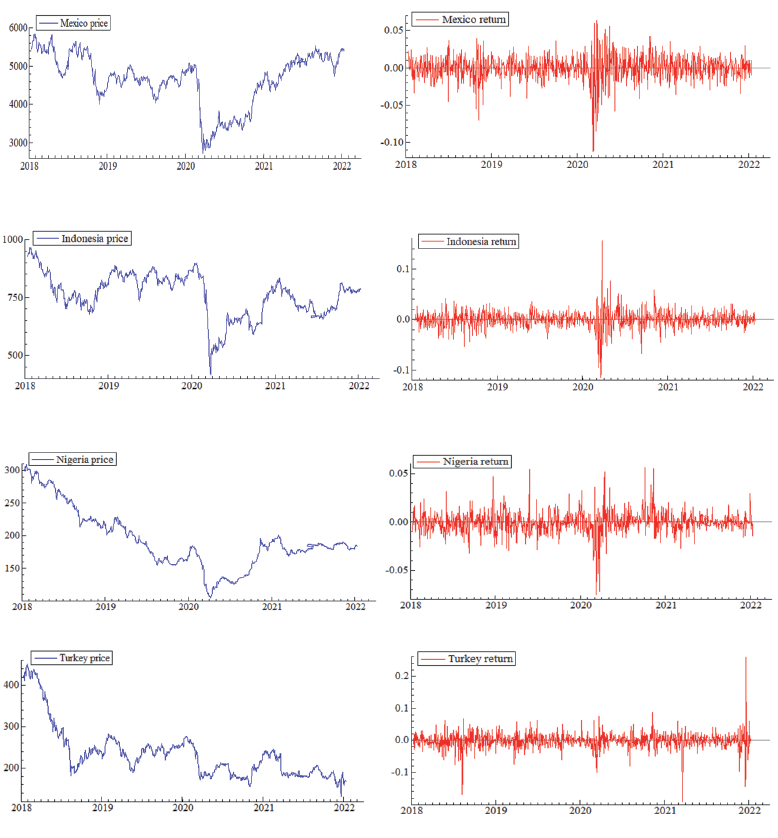
Figure 2 displays the autocorrelation plots of the MINT stock price-return series. From these plots, it is seen that the return to the mean is quite slow. Based on this fact, the possibility of the existence of long memory in the price series or the change series can be mentioned.

Figure 2
The Autocorrelation Plots of the MINT Stock Price-Return Series

 

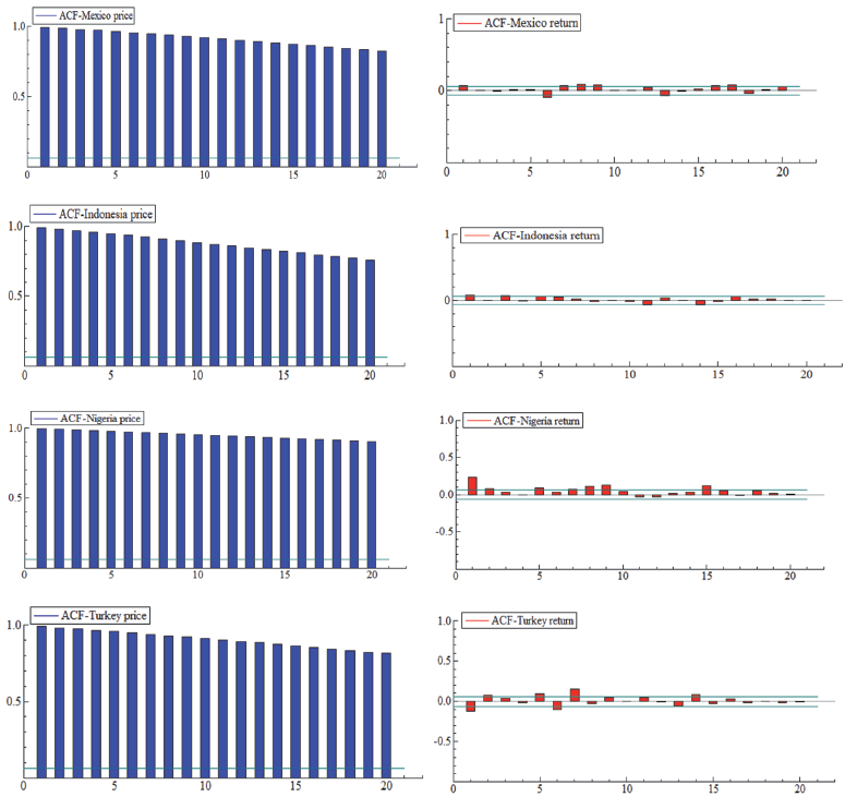
Table 2 reports the descriptive statistics for the MINT stock returns. The results show that the highest return belongs to Mexico, and the lowest return belongs to Turkey, while the highest standard deviation belongs to Mexico, and the lowest standard deviation belongs to Nigeria. The variables’ skewness values indicate negative asymmetry, and the variables’ high kurtosis values indicate the fat tails, or outliers. The non-normality is also verified by the rejection of the Jarque-Bera (JB) test statistics null hypothesis at the 1% level of significance. The heteroscedasticity is verified by the rejection of the ARCH-LM test statistics null hypothesis of no conditional heteroscedasticity at the 1% level of significance. The Augmented Dickey-Fuller (1979) (ADF), Phillips–Perron (PP) (1988), Kwiatkowski, Phillips, Schmidt, and Shin (KPSS) (1992) tests show that all variables are stationary. The serial correlation is verified by the rejection of the Ljung-Box test statistics null hypothesis at the 1% level of significance.

Table 2
The Descriptive Statistics for the MINT Stock Returns

	Mexico	Indonesia	Nigeria	Turkey
Mean	0.0000	-0.0001	-0.0004	-0.0008
S.dev	0.0242	0.0163	0.0107	0.0234
Skewness	-0.8853	-0.0437	-0.2475	0.0046
Kurtosis	8.9322	15.9831	10.7138	22.6515
ADF	-30.0975a	-29.6419a	-25.4179a	-32.1928a
PP test	-30.2287a	-29.8856a	-26.0382a	-32.2578a
KPSS test	0.1528a	0.0722a	0.3215a	0.1019a
p-value (JB)	1665.645a	7325.749a	2591.578a	16782.888a
ARCH(5)	93.9771a	71.1897a	18.8111a	90.6955a
Q(20)	25.0016a	16.2864a	26.3441a	25.6475a

Note. (^a), (^b) and (^c) denote statistical significance at 1%, 5%, and 10 % levels. The ARCH(5) denotes the ARCH test statistic with lag 5. The Q(20) is the Ljung-Box test statistic for return residuals 20 lag.

4. Empirical Findings

4.1 Estimation Results of ARFIMA Models

This study estimates some specifications of the ARFIMA models for different lags (p,q) under the assumption of normal distribution. Cheung (1993) suggests the use of maximum likelihood procedures (p,q) ϵ (0,1,2) to estimate the ARFIMA (p,d,q) models. Following Cheung (1993), firstly, various possible combinations are carried out from ARFIMA (0,d,0) to ARFIMA(2,d,2), and the appropriate model structure is determined by considering the significance of the coefficient, the model selection criteria including Log-likelihood [Ln(L)] value and Akaike Information Criterion (AIC).

Table 3 indicates estimation results and diagnostic statistics of the MINT ARFIMA (p, d,q) models. According to the significance of the coefficient, the model selection criteria including Ln(L) value and AIC, the Mexico stock returns prefer the ARFIMA (2,d,2) model, which gives the smallest AIC (-5.3576) and the largest Ln(L) (2801.019) for a long memory process. The Indonesia stock returns prefer the ARFIMA (2,d,1) model, which gives the smallest AIC (-5.2848) and the largest Ln(L) (2763.036) for a long memory process. The Nigeria stock returns prefer the ARFIMA (2,d,2) model, which gives the smallest AIC (-6.2116) and the largest Ln(L) (3246.388) for a long memory process. The Turkey stock returns prefer the ARFIMA (1,d,0) model, which gives the smallest AIC (-4.6731) and the largest Ln(L) (2441.232) for a long memory process. The ARFIMA (p,d,q) models with d ϵ (0, 0.5) statistically significant at 1% and 10% indicate long-term memory for the MINT stock returns. Thus, this situation shows a predictable behavior of stock returns for the MINT, which is consistent with the FMH.

Table 3
The Estimation Results of the ARFIMA (p,d,q) for MINT

(p,d,q)	(0,d,0)	(0,d,1)	(0,d,2)	(1,d,0)	(1,d,1)	(1,d,2)	(2,d,0)	(2,d,1)	(2,d,2)
Panel A: Mexico return
Cons.	0.0005 (0.952)	0.0005 (0.958)	0.0005 (0.954)	0.0005 (0.958)	0.0005 (0.955)	0.0005 (0.941)	0.0005 (0.954)	0.0005 (0.993)	0.0005 (0.945)
AR-1	-	-	-	0.0419 (0.411)	-0.8222 (0.000)a	0.5284 (0.002)a	0.0226 (0.697)	1.2636 (0.000)a	1.5934 (0.000)a
AR-2	-	-	-	-	-	-	-0.0256 (0.507)	-0.2921 (0.119)	-0.9589 (0.000)a
d	0.0544 (0.031)b	0.0274 (0.477)	0.0495 (0.378)	0.0279 (0.490)	0.0419 (0.118)	0.1509 (0.217)	0.0481 (0.339)	-0.3783 (0.164)	0.0759 (0.000)a
MA-1	-	0.0437 (0.375)	0.0202 (0.756)	-	0.8511 (0.000)a	-0.6095 (0.005)a	-	-0.8191 (0.000)a	-1.6118 (0.000)a
MA-2	-	-	-0.0253 (0.564)	-	-	-0.0353 (0.418)	-	-	0.9595 (0.000)a
Ln(L)	2795.30	2795.67	2795.84	2795.64	2796.52	2796.47	2795.86	2798.35	2801.01
AIC	-5.3543	-5.3531	-5.3515	-5.3531	-5.3528	-5.3508	-5.3516	-5.3544	-5.3576
ARCH (5)	90.065 (0.000)a	91.794 (0.000)a	90.031 (0.000)a	91.785 (0.000)a	89.267 (0.000)a	88.149 (0.000)a	90.082 (0.000)a	88.278 (0.000)a	80.469 (0.000)a
Q(20)	55.163 (0.000)a	54.034 (0.000)a	53.057 (0.000)a	54.160 (0.000)a	51.020 (0.000)a	49.642 (0.000)a	53.000 (0.000)a	49.077 (0.000)a	45.238 (0.000)a
Panel B: Indonesia return
Cons.	-0.0001 (0.851)	-0.0001 (0.827)	-0.0001 (0.862)	-0.0001 (0.830)	-0.0001 (0.829)	-0.0001 (0.857)	-0.0001 (0.867)	-0.0001 (0.859)	-0.0001 (0.675)
AR-1	-	-	-	0.0384 (0.468)	-0.6999 (0.000)a	-0.6275 (0.000)a	-0.0093 (0.883)	-0.6869 (0.000)a	0.2216 (0.258)
AR-2	-	-	-	-	-	-	-0.0519 (0.217)	-0.0531 (0.310)	0.5077 (0.000)a
d	0.0698 (0.006)a	0.0419 (0.316)	0.0881 (0.140)	0.0447 (0.296)	0.0452 (0.109)	0.0787 (0.110)	0.0939 (0.101)	0.0805 (0.080)c	-0.1712 (0.222)
MA-1	-	0.0437 (0.414)	0.0009 (0.989)	-	0.7545 (0.000)a	0.6386 (0.001)a	-	0.6948 (0.000)a	0.0347 (0.828)
MA-2	-	-	-0.0532 (0.213)	-	-	-0.0510 (0.361)	-	-	-0.4639 (0.000)a
Ln(L)	2758.85	2759.17	2759.96	2759.12	2761.41	2761.81	2759.86	2763.03	2763.03
AIC	-5.2844	-5.2831	-5.2827	-5.2830	-5.2855	-5.2844	-5.2825	-5.2848	-5.2845
ARCH (5)	55.701 (0.000)a	61.975 (0.000)a	58.594 (0.000)a	61.085 (0.000)a	57.516 (0.000)a	51.126 (0.000)a	57.082 (0.000)a	50.242 (0.000)a	51.893 (0.000)a
Q(20)	31.244 (0.000)a	30.647 (0.031)b	28.117 (0.043)b	30.771 (0.030)b	25.687 (0.080)c	24.685 (0.075)c	28.278 (0.041)b	24.574 (0.077)c	23.930 (0.066)c
Panel C: Nigeria return
Cons.	-0.0005 (0.631)	-0.0005 (0.554)	-0.0005 (0.515)	-0.0005 (0.544)	-0.0005 (0.537)	-0.0005 (0.000)a	-0.0005 (0.529)	-0.0005 (0.527)	-0.0005 (0.590)
AR-1	-	-	-	0.0679 (0.201)	0.1350 (0.697)	0.0383 (0.983)	0.0756 (0.209)	-0.0757 (0.905)	-0.2367 (0.000)a
AR-2	-	-	-	-	-	-	0.0104 (0.783)	0.0245 (0.684)	-0.9180 (0.000)a
d	0.1700 (0.000)a	0.1313 (0.000)a	0.1111 (0.027)b	0.1260 (0.000)a	0.1220 (0.012)b	0.1186 (0.027)b	0.1178 (0.023)b	0.1168 (0.020)b	0.1501 (0.000)a
MA-1	-	0.0614 (0.190)	0.0828 (0.159)	-	-0.0631 (0.846)	0.0359 (0.984)	-	0.1522 (0.808)	0.2720 (0.000)a
MA-2	-	-	0.0263 (0.571)	-	-	-0.0001 (0.999)	-	-	0.9444 (0.000)a
Ln(L)	3241.02	3241.83	3241.99	3241.87	3241.89	3258.05	3241.91	3241.93	3246.38
AIC	-6.2090	-6.2086	-6.2070	-6.2087	-6.2068	-6.2359	-6.2069	-6.2050	-6.2116
ARCH (5)	56.232 (0.000)a	54.697 (0.000)a	52.652 (0.000)a	54.285 (0.000)a	53.857 (0.000)a	53.927 (0.000)a	53.402 (0.000)a	53.182 (0.000)a	51.510 (0.000)a
Q(20)	45.149 (0.000)***	41.943 (0.001)a	41.781 (0.001)a	41.850 (0.001)a	41.894 (0.000)a	41.764 (0.000)a	41.949 (0.000)a	41.888 (0.000)a	39.226 (0.000)a
Panel D: Turkey return
Cons.	-0.0003 (0.510)	-0.0004 (0.781)	-0.0004 (0.735)	-0.0004 (0.732)	-0.0003 (0.152)	-0.0003 (0.472)	-0.0003 (0.132)	-0.0003 (0.141)	-0.0003 (0.142)
AR-1	-	-	-	-0.2240 (0.000)a	0.9781 (0.000)a	0.8985 (0.000)a	0.7449 (0.000)a	0.8715 (0.000)a	0.8180 (0.100)
AR-2	-	-	-	-	-	-	0.2367 (0.000)a	0.1075 (0.443)	0.1596 (0.742)
d	-0.0271 (0.221)	0.1483 (0.000)a	0.1057 (0.079)c	0.1045 (0.000)a	-0.7689 (0.352)	-0.1970 (0.452)	-0.8699 (0.355)	-0.8134 (0.497)	-0.8089 (0.485)
MA-1	-	-0.2613 (0.000)a	-0.2268 (0.001)a	-	-0.3336 (0.000)a	-0.8243 (0.000)	-	-0.1878 (0.355)	-0.1389 (0.771)
MA-2	-	-	0.0462 (0.217)	-	-	0.0698 (0.479)	-	-	-0.0175 (0.914)
Ln(L)	2429.17	2440.40	2441.15	2441.23	2442.69	2441.70	2442.57	2443.01	2443.02
AIC	-4.6523	-4.6719	-4.6714	-4.6731	-4.6743	-4.6705	-4.6741	-4.6730	-4.6711
ARCH (5)	119.59 (0.000)a	87.393 (0.000)a	80.495 (0.000)a	79.245 (0.000)a	86.164 (0.000)a	86.203 (0.000)a	78.172 (0.000)a	81.043 (0.000)a	80.875 (0.000)a
Q(20)	82.433 (0.000)a	44.838 (0.000)a	40.705 (0.000)a	40.516 (0.001)a	43.975 (0.000)a	44.437 (0.000)a	40.495 (0.001)a	40.984 (0.000)a	40.970 (0.000)a

Note. The values in parentheses indicate the probability value. (^a), (^b) and (^c) denote statistical significance at 1%, 5%, and 10 % levels. The ARCH(5) denotes the ARCH test statistic with lag 5. The Q(20) is the Ljung-Box test statistics with 20 degrees of freedom based on the standardized residuals.

However, the diagnostic statistics show some limitations in constructing the ARFIMA model in the MINT stock return series. For instance, the heteroscedasticity is verified by the rejection of the ARCH test statistics null hypothesis of no conditional heteroscedasticity in the standardized residuals. The serial correlation is verified by the rejection of the Ljung-Box test statistics null hypothesis at the 1% level of significance. Therefore, these statistics imply that modeling the returns level alone is not suitable for capturing the presence of the long memory property in the MINT stock markets.

4.2 Estimation Results of the ARFIMA–FIGARCH Type Models

The long memory dynamics are commonly observed in both the conditional mean and variance. Thus, it can be analyzed as the dual long memory property in both the conditional mean and variance (Kang & Yoon, 2007). Table 4 indicates the estimation results of the ARFIMA-FIGARCH, ARFIMA-FIAPARCH, and ARFIMA-FIEGARCH models for the Mexico stock returns under the normal and S-student-t distributions for Mexico, and all significant distributions of the ARFIMA-FIGARCH, ARFIMA-FIAPARCH and, ARFIMA-FIEGARCH models.

Table 4
Estimation Results of the ARFIMA-FIGARCH Type Models for Mexico

	ARFIMA(2,d,2)- FIGARCH (1,d,1)		ARFIMA(2,d,2)- FIAPARCH(1,d,1)		ARFIMA(2,d,2)- FIEGARCH(1,d,1)
	Normal	S-student-t	Normal	S-student-t	Normal	S-student-t
Cst(M)	0.0002 (0.577)	0.0001 (0.522)	0.000 (0.902)	0.0000 (0.971)	0.0008 (0.722)	0.0003 (0.375)
d-Arfima	-0.0746 (0.809)	-0.0907 (0.339)	-0.0547 (0.657)	-0.085 (0.348)	-0.2839 (0.000)a	-0.2054 (0.155)
AR(1)	0.9310 (0.115)	0.8086 (0.047)b	0.8643 (0.008)a	0.7827 (0.170)	1.0000 (0.000)a	1.0000 (0.039)b
AR(2)	-0.1368 (0.505)	-0.1469 (0.414)	-0.1535 (0.496)	-0.1460 (0.453)	-0.1003 (0.066)c	-0.14025 (0.604)
MA(1)	-0.7670 (0.024)b	-0.6350 (0.150)	-0.7297 (0.035)b	-0.617 (0.303)	-0.6552 (0.000)a	-0.7207 (0.102)
MA(2)	0.0265 (0.891)	0.0440 (0.767)	0.0574 (0.801)	0.0544 (0.713)	-0.0780 (0.056)c	-0.0208 (0.884)
Cst(V) x 10^4	2.3870 (0.011)b	1.9322 (0.001)a	10.9067 (0.343)	7.5067 (0.359)	0.0000 (1.000)	0.0000 (1.000)
d-Figarch	0.3543 (0.000)a	0.2958 (0.000)a	0.2947 (0.000)a	0.2405 (0.000)a	0.6657 (0.000)a	0.6347 (0.000)a
ARCH (Phi1)	-0.2223 (0.091)c	-0.1770 (0.142)	-0.1853 (0.217)	-0.1161 (0.450)	-0.6914 (0.000)a	0.3284 (0.409)
GARCH (Beta1)	0.0454 (0.749)	0.0536 (0.695)	0.0489 (0.748)	0.0823 (0.612)	0.9066 (0.000)a	0.9895 (0.000)a
Asym­metry	-	-0.1104 (0.009)b	-	-0.1134 (0.006)b	-	0.0829 (0.020)b
Tail	-	9.8687 (0.000)a	-	10.1755 (0.000)a	-	5.7986 (0.000)a
APARCH (Gamma1)	-	-	0.3177 (0.114)	0.4192 (0.075)c	-	-
APARCH (Delta)	-	-	1.6437 (0.000)a	1.6675 (0.000)a	-	-
EGARCH (Theta1)	-	-	-	-	-0.0103 (0.000)a	-0.0163 (0.510)
EGARCH (Theta2)	-	-	-	-	0.4943 (0.000)a	0.4019 (0.000)a
Ln(L)	2969.153	2982.228	2973.828	2986.935	2886.446	2905.953
AIC	-5.6743	-5.6955	-5.6794	-5.5454	-5.5118	-5.5454
ARCH(5)	0.7977 (0.551)	1.1255 (0.344)	0.75797 (0.580)	1.8501 (0.100)	1.7026 (0.131)	1.8501 (0.100)
Q(20)	2.3038 (0.218)	26.6330 (0.186)	15.7637 (0.609)	21.3433 (0.262)	22.1198 (0.226)	21.3433 (0.262)

Note. The values in parentheses indicate the probability value. (^a), (^b) and (^c) denote statistical significance at 1%, 5%, and 10 % levels. The ARCH(5) denotes the ARCH test statistic with lag 5. The Q(20) is the Ljung-Box test statistics with 20 degrees of freedom based on the standardized residuals.

To capture the dual long memory property, the ARFIMA(2,d,2)-FIGARCH(1,d,1), ARFIMA(2,d,2)-FIAPARCH(1,d,1), and ARFIMA(2,d,2)-FIEGARCH(1,d,1) model specifications are estimated, and the model parameters are presented in Table 4. The ARFIMA(2,d,2)-FIEGARCH(1,d,1) specification is found to be the best model for capturing the dual long memory property in the returns and volatility of the Mexico stock. In the estimates of the ARFIMA(2,d,2)-FIEGARCH(1,d,1) model, both the long memory parameters d-ARFIMA and d-FIGARCH are significantly different from zero, indicating that the dual long memory property is prevalent in the return and volatility of the Mexico stock. The results also show that the normal distribution performs better than the S-student-t distribution. In the ARFIMA (2,d,2)-FIEGARCH(1,d,1) model, the EGARCH (Theta1) and EGARCH (Theta2) parameters indicate the sign and magnitude effects, respectively. The EGARCH (Theta1) parameter is negative and statistically significant at the 1% level. This means that negative information shocks reaching the market cause more volatility than positive information shocks. The EGARCH (Theta2) parameter is also statistically significant at the 1% level.

Table 5
Estimation Results of the ARFIMA-FIGARCH Type Models for Indonesia

	ARFIMA(2,d,1)-FIGARCH(1,d,1)		ARFIMA(2,d,1)-FIAPARCH(1,d,1)		ARFIMA(2,d,1)-FIEGARCH(1,d,1)
	Normal	S-student-t	Normal	S-student-t	Normal
Cst(M)	0.0000 (0.893)	0.0004 (0.655)	-0.0001 (0.692)	-0.0000 (0.826)	0.0002 (0.323)
d-Arfima	-0.3188 (0.016)b	-0.0027 (0.957)	-0.0131 (0.823)	0.0033 (0.948)	0.0219 (0.725)
AR(1)	1.0639 (0.000)a	-0.6177 (0.000)a	-0.5243 (0.000)a	-0.6050 (0.000)a	-0.5283 (0.000)a
AR(2)	-0.1523 (0.034)b	-0.0879 (0.063)b	-0.0320 (0.604)	-0.0843 (0.092)c	-0.0666 (0.237)
MA(1)	-0.7518 (0.000)a	0.5968 (0.000)a	0.5685 (0.000)a	0.5917 (0.000)a	0.5320 (0.000)a
Cst(V) x 10^4	2.7116 (0.043)b	3.5535 (0.062)c	0.1297 (0.776)	0.8168 (0.549)	-8.8055 (0.000)a
d-Figarch	0.3709 (0.001)a	0.3381 (0.000)a	0.1200 (0.116)	0.2336 (0.015)b	0.7895 (0.000)a
ARCH (Phi1)	0.2349 (0.270)	-0.1805 (0.425)	-0.6999 (0.000)a	0.0916 (0.832)	0.0706 (0.842)
GARCH (Beta1)	0.4117 (0.130)	-0.0187 (0.942)	-0.7341 (0.000)a	0.1682 (0.709)	-0.5302 (0.000)a
Asymmetry	-	-0.0195 (0.595)	-	-0.0142 (0.689)	-
Tail	-	4.9119 (0.000)a	-	6.1832 (0.000)a	-
APARCH (Gamma1)	-	-	0.6065 (0.020)b	0.4339 (0.000)a	-
APARCH (Delta)	-	-	2.0351 (0.000)a	1.7227 (0.000)a	-
EGARCH (Theta1)	-	-	-	-	-0.1907 (0.000)a
EGARCH (Theta2)	-	-	-	-	0.2070 (0.025)b
Ln(L)	2973.739	2997.926	2992.312	3007.229	2982.791
AIC	-5.6850	-5.7275	-5.7168	-5.7415	-5.6985
ARCH(5)	0.2173 (0.955)	0.39175 (0.854)	0.6537 (0.658)	0.17911 (0.970)	2.7259 (0.818)
Q(20)	8.7706 (0.964)	11.0418 (0.892)	8.6403 (0.967)	6.4645 (0.993)	26.3755 (0.891)

Note. The values in parentheses indicate the probability value. (^a), (^b) and (^c) denote statistical significance at 1%, 5%, and 10 % levels. The ARCH(5) denotes the ARCH test statistic with lag 5. The Q(20) is the Ljung-Box test statistics with 20 degrees of freedom based on the standardized residuals.

Table 5 reports the estimation results of the ARFIMA-FIGARCH type models for the Indonesia stock returns under the normal and S-student-t and all significant distributions of the ARFIMA-FIGARCH type models. The ARFIMA(2,d,1)-FIAPARCH(1,d,1) specification is found to be the best model for capturing the dual long memory property in the returns and volatility of the Indonesia stock, according to the Ln(L) and AIC. In the estimates of the ARFIMA(2,d,1)-FIAPARCH(1,d,1) model, both the long memory parameters d-ARFIMA and d-FIGARCH are significantly different from zero, indicating that the dual long memory property is prevalent in the return and volatility of the Indonesia stock. The results also show that the S-student-t distribution performs better than the normal distribution. The APARCH(Gamma1) is the parameter which considers the leverage effect. The APARCH(Gamma1) parameter is positive and statistically significant at the 1% level. This means that negative information shocks reaching the market cause more volatility than positive information shocks. The APARCH(Delta) parameter is also statistically significant at the 1% level. The tail parameter is statistically significant at the 1% level. This means that the presence of the fat tail feature is parallel with the result obtained in the descriptive statistics.

Table 6 reports the estimation results of the ARFIMA-FIGARCH type models for the Nigeria stock returns under the normal and S-student-t and all significant distributions of the ARFIMA-FIGARCH type models. The ARFIMA(2,d,2)-FIAPARCH(1,d,1) specification is found to be the best model for capturing the dual long memory property in the returns and volatility of the Indonesia stock, according to the Ln(L) and AIC. In the estimates of the ARFIMA(2,d,2)-FIAPARCH(1,d,1) model, both the long memory parameters d-ARFIMA and d-FIGARCH are significantly different from zero, indicating that the dual long memory property is prevalent in the return and volatility of the Indonesia stock. The results also show that the S-student-t distribution performs better than the normal distribution. The APARCH(Delta) parameter is also statistically significant at the 1% level. The tail parameter is statistically significant at the 1% level. This means that the presence of the fat tail feature is parallel with the result obtained in the descriptive statistics.

Table 6
Estimation Results of the ARFIMA-FIGARCH Type Models for Nigeria

	ARFIMA(2,d,2)-FIGARCH(1,d,1)		ARFIMA(2,d,2)-FIAPARCH(1,d,1)		ARFIMA(2,d,2)-FIEGARCH(1,d,1)
	Normal	S-student-t	Normal	S-student-t	Normal
Cst(M)	-0.0002 (0.656)	-0.0004 (0.382)	-0.0005 (0.521)	-0.0004 (0.294)	0.0006 (0.264)
d-Arfima	0.1156 (0.000)a	0.0826 (0.002)a	0.113 (0.000)a	0.0784 (0.002)a	0.0491 (0.000)a
AR(1)	0.2810 (0.000)a	0.2918 (0.000)a	0.2759 (0.000)a	0.2943 (0.000)a	-0.7310 (0.000)a
AR(2)	-0.6260 (0.000)a	-0.8481 (0.000)a	-0.9227 (0.000)a	-0.8847 (0.000)a	-0.1298 (0.000)a
MA(1)	-0.2497 (0.000)a	-0.2485 (0.000)a	0.2459 (0.000)a	-0.2560 (0.000)a	0.8893 (0.000)a
MA(2)	0.9293 (0.000)a	0.8349 (0.000)a	0.9281 (0.000)a	0.8785 (0.000)a	0.2358 (0.000)a
Cst(V) x 10^4	0.0470 (0.236)	0.0786 (0.142)	1.2579 (0.623)	16.5145 (0.476)	0.0000 (1.000)
d-Figarch	0.4533 (0.213)	0.5546 (0.000)a	0.6486 (0.139)	0.4493 (0.000)a	0.2927 (0.186)
ARCH (Phi1)	0.3687 (0.045)b	0.3868 (0.019)	0.3173 (0.058)	0.4492 (0.098)c	-0.5540 (0.024)b
GARCH (Beta1)	0.6247 (0.029)b	0.6391 (0.000)a	0.7625 (0.010)b	0.6339 (0.002)a	0.9831 (0.000)a
Asymmetry	-	0.0264 (0.423)	-	0.0327 (0.329)	-
Tail	-	3.3272 (0.000)a	-	3.4108 (0.000)a	-
APARCH (Gamma1)	-	-	0.0239 (0.876)	0.1236 (0.289)	-
APARCH (Delta)	-	-	1.3502 (0.000)a	1.6976 (0.000)a	-
EGARCH (Theta1)	-	-	-	-	-0.0188 (0.593)
EGARCH (Theta2)	-	-	-	-	0.4149 (0.000)a
Ln(L)	3363.932	3449.362	3368.566	3453.976	3258.990
AIC	-6.4313	-6.5912	-6.4363	-6.5963	-6.2262
ARCH(5)	0.5587 (0.731)	0.7702 (0.571)	0.4957 (0.779)	0.5896 (0.707)	0.6469 (0.663)
Q(20)	8.4315 (0.971)	8.6869 (0.966)	8.6641 (0.967)	9.2570 (0.953)	10.2525 (0.923)

Note. The values in parentheses indicate the probability value. (^a), (^b) and (^c) denote statistical significance at 1%, 5%, and 10 % levels. The ARCH(5) denotes the ARCH test statistic with lag 5. The Q(20) is the Ljung-Box test statistics with 20 degrees of freedom based on the standardized residuals.

Table 7
Estimation Results of the ARFIMA-FIGARCH Type Models for Turkey

	ARFIMA (1,d,0)-FIGARCH(1,d,1)		ARFIMA (1,d,0)-FIAPARCH(1,d,1)		ARFIMA (1,d,0)-FIEGARCH(1,d,1)
	Normal	S-student-t	Normal	S-student-t	Normal	S-student-t
Cst(M)	0.0001 (0.806)	-0.0000 (0.907)	-0.0004 (0.467)	-0.0002 (0.559)	0.0000 (0.899)	-0.0005 (0.317)
d-Arfima	0.0072 (0.864)	-0.0481 (0.234)	0.0005 (0.990)	-0.0329 (0.417)	0.0142 (0.727)	-0.0273 (0.000)a
AR(1)	-0.0104 (0.843)	0.0259 (0.623)	0.0188 (0.745)	0.0308 (0.567)	0.009 (0.850)	0.0315 (0.000)a
Cst(V) x 10^4	0.5216 (0.110)	0.4757 (0.121)	4.2876 (0.465)	2.0603 (0.492)	-7.705 (0.000)a	-8.117 (0.000)a
d-Figarch	0.2726 (0.014)b	0.2434 (0.001)a	0.1860 (0.013)b	0.1805 (0.009)a	0.6408 (0.000)a	0.6092 (0.000)a
ARCH (Phi1)	-0.3215 (0.202)	-0.2083 (0.443)	-0.3147 (0.238)	-0.3059 (0.216)	1.0745 (0.100)	1.0529 (0.090)c
GARCH (Beta1)	-0.1061 (0.690)	-0.0353 (0.906)	-0.1836 (0.517)	-0.1812 (0.488)	-0.1997 (0.168)	-0.1603 (0.145)
Asymmetry		0.1089 (0.013)b		-0.0965 (0.026)b		-0.0300 (0.332)
Tail		7.3963 (0.000)a		8.1067 (0.000)a		7.6201 (0.000)a
APARCH (Gamma1)				0.5493 (0.023)b
APARCH (Delta)				1.7149 (0.000)a
EGARCH (Theta1)					-0.1315 (0.006)a	-0.1196 (0.005)a
EGARCH (Theta2)					0.1398 (0.004)a	0.1511 (0.006)a
Ln(L)	2634.776	2660.280	2647.485	2666.985	2642.189	2662.301
AIC	-5.0388	-5.0839	-5.0594	-5.0929	-5.0492	-5.0839
ARCH(5)	0.6622 (0.652)	0.9973 (0.418)	0.4370 (0.822)	0.5635 (0.728)	1.2296 (0.293)	1.7209 (0.127)
Q(20)	39.7615 (0.002)a	46.8295 (0.000)a	20.6145 (0.299)	23.2264 (0.182)	27.5731 (0.168)	34.5810 (0.110)

Note. The values in parentheses indicate the probability value. (^a), (^b) and (^c) denote statistical significance at 1%, 5%, and 10 % levels. The ARCH(5) denotes the ARCH test statistic with lag 5. The Q(20) is the Ljung-Box test statistics with 20 degrees of freedom based on the standardized residuals.

Table 7 reports the estimation results of the ARFIMA-FIGARCH type models for the Turkey stock returns under the normal and S-student-t and all significant distributions of the ARFIMA-FIGARCH type models. The ARFIMA(1,d,0)-FIEGARCH(1,d,1) specification is found to be the best model for capturing the dual long memory property in the returns and volatility of the Turkey stock. In the estimates of the ARFIMA(1,d,0)-FIEGARCH(1,d,1) model, both the long memory parameters d-ARFIMA and d-FIGARCH are significantly different from zero, indicating that the dual long memory property is prevalent in the return and volatility of the Turkey stock. The results also show that the S-student-t distribution performs better than the normal distribution. The EGARCH (Theta1) parameter is negative and statistically significant at the 1% level. This means that negative information shocks reaching the market cause more volatility than positive information shocks. The EGARCH (Theta2) parameter is also statistically significant at the 1% level.

In summary, the empirical findings indicate that long memory is reported for both the conditional mean and conditional variance in the MINT stock returns. The long memory in the returns and volatility implies that the MINT stock prices follow a predictable behavior that is consistent with the FMH. Besides, self-similarity among fractal market conditions can be seen as market factors impacting investment decisions for the MINT stock market participants. Van Quang (2005), Aygören (2008), Ural and Demireli (2009), Panas and Ninni (2010), Sensoy (2013), Cevik andTopaloglu (2014), Kumar and Bandi (2015), Doorasamy and Sarpong (2018), Aslam et al. (2020) conclude that the stock market prices exhibit long memory, and the FMH is valid. This study is consistent with the above findings, but inconsistent with Günay (2015).

The EGARCH(Theta1) and APARCH(Gamma1) parameters indicate the impact of the information reaching the market. It is seen that the EGARCH(Theta1) parameters of Mexico and Turkey are negative and statistically significant. It is seen that the APARCH(Gamma1) parameter of Indonesia is positive and statistically significant, and the APARCH(Gamma1) parameter of Nigeria is positive and statistically insignificant. Thus, negative information shocks reaching the Mexico, Indonesia, and Turkey stock markets cause more volatility than positive information shocks. The fact that the ARCH(Phi1) parameter, which represents the impact of past shocks, is close to one and is statistically significant indicates that the impact of past shocks is strong, while the negative GARCH(Beta1) parameter, which represents volatility, indicates that the permanence of the impact is weak. Among the MINT stock markets, Turkey has the highest ARCH(Phi1) parameter, but the negative GARCH(Beta1) parameter indicates that the permanence of the effect is weak. These findings can give insight to both domestic and foreign capital investors and portfolio managers. If investors want to invest in the least risky stock market, they may prefer the Turkey stock market. Similarly, they may prefer the Nigeria stock market as the riskiest market.

5. Conclusions

This study investigates the market efficiency of the MINT stock markets based on the FMH. The MINT stock return series are modeled using the ARFIMA models. The ARFIMA models indicate the existence of long memory in the MINT stock return series. However, the diagnostic statistics show some limitations in constructing the ARFIMA model in the MINT stock return series. For instance, the heteroscedasticity is verified by the rejection of the ARCH test statistics null hypothesis of no conditional heteroscedasticity in the standardized residuals. The serial correlation is verified by the rejection of the Ljung-Box test statistics null hypothesis at the 1% level of significance. Therefore, these statistics imply that modeling the returns level alone is not suitable for capturing the presence of the long memory property in the MINT stock return series. For this reason, this study tests the dual long memory property of the MINT stock markets. Thus, in this study, the ARFIMA-FIGARCH type models are used to test the property of long memory in the MINT stock returns and volatility. The ARFIMA-FIGARCH type models are estimated under both the normal and S-student-t distributions. The empirical findings show that the long memory is reported for both the conditional mean and conditional variance in the MINT stock returns. Besides, the estimation results also show that the S-Student-t distribution outperforms the normal distribution, but not in Mexico. The existence of long memory means that the fractal market conditions are valid in both the MINT stock returns and volatility series.

In summary, the empirical findings show that long memory is reported for the MINT stock returns. The long memory in the mean implies that the MINT stock prices follow a predictable behavior that is consistent with the FMH. Thus, investors who seek profit can make predictions about the prices of the future period by using the past prices of the MINT stock market with many analysis methods, mainly technical and fundamental analysis, and they can earn abnormal returns from the market, although not always. The long memory in the volatility implies that uncertainty or risk is an important factor in the formation of price movements in the MINT stock prices. Moreover, the MINT stock prices consist of the impact of shocks and news that occurred in the recent past. For this reason, studying the long memory behavior in the MINT stock prices may be important for investors, portfolio managers, financial institutions, portfolio diversification, portfolio optimization, risk management, hedging, price discovery, and investment decisions. Besides, these findings would help regulators. They should try to understand the sources of long memory in the market to increase efficiency.

References

Adebayo, T. S., Awosusi, A. A., & Adeshola, I. (2020). Determinants of CO₂ Emissions in Emerging Markets: An Empirical Evidence from MINT Economies. International Journal of Renewable Energy Development, 9(3), 411–422.

Adubisi, O. D., Abdulkadir, A., Farouk, U. A., & Chiroma, H. (2022). The exponentiated half logistic skew-t distribution with GARCH-type volatility models. Scientific African, 16, e01253. https://doi.org/10.1016/j.sciaf.2022.e01253

Arouxet, M. B., Bariviera, A. F., Pastor, V. E., & Vampa, V. (2022). Covid-19 impact on cryptocurrencies: Evidence from a wavelet-based Hurst exponent. Physica A: Statistical Mechanics and its Applications, 596, 127170. https://doi.org/10.1016/j.physa.2022.127170

Aslam, F., Latif, S., & Ferreira, P. (2020). Investigating Long-Range Dependence of Emerging Asian Stock Markets Using Multifractal Detrended Fluctuation Analysis. Symmetry, 12(7), 1157. https://doi.org/10.3390/sym12071157

Aygören, H. (2008). İstanbul menkul kıymetler borsasının fractal analizi. Dokuz Eylül Üniversitesi İktisadi İdari Bilimler Fakültesi Dergisi, 23(1), 125–134.

Bachelier, L. (1900). The Random Character of Stock Market Prices. Cambridge: MIT Press.

Baillie, R. T., Bollerslev, T., & Mikkelsen, H. O. (1996). Fractionally Integrated Generalized Autoregressive Conditional Heteroscedasticity. Journal of Econometrics, 74, 3–30.

Bam, N., Thagurathi, R. K., & Shrestha, B. (2018). Stock Price Behavior of Nepalese Commercial Banks: Random Walk Hypothesis. Journal of Business and Management, 5, 42–52. https://doi.org/10.3126/jbm.v5i0.27387

Blackledge, J., & Lamphiere, M. (2021). A Review of the Fractal Market Hypothesis for Trading and Market Price Prediction. Mathematics, 10(1), 117. https://doi.org/10.3390/math10010117

Brătian, V., Acu, A. M., Oprean-Stan, C., Dinga, E., & Ionescu, G. M. (2021). Efficient or Fractal Market Hypothesis? A Stock Indexes Modelling Using Geometric Brownian Motion and Geometric Fractional Brownian Motion. Mathematics, 9(22), 2983. https://doi.org/10.3390/math9222983

Bollerslev, T., & Mikkelsen, H. O. (1996). Modelling and pricing long memory in stock market volatility. Journal of Econometrics, 73, 151–184. https://doi.org/10.1016/0304-4076(95)01736-4

Cevik, E. I., & Topaloglu, G. (2014). Volatilitede uzun hafiza ve yapisal kirilma: borsa istanbul örneği. Balkan Sosyal Bilimler Dergisi, 3(6), 40–55.

Cheung, Y. W. (1993). Long memory in foreign-exchange rates. Journal of Business & Economic Statistics, 11(1), 93–101. https://doi.org/10.1080/07350015.1993.10509935

Cowles, A. (1933). Can stock market forecasters forecast? Econometrica, 1(3), 309–324.

Dickey, D. A., & Fuller, W. A. (1979). Distribution of the estimators for autoregressive time series with a unit root. Journal of the American Statistical Association, 74(366a), 427–431.

Demirel, M., & Unal, G. (2020). Applying multivariate-fractionally integrated volatility analysis on emerging market bond portfolios. Financial Innovation, 6(1), 1–29. https://doi.org/10.1186/s40854-020-00203-3

Doorasamy, M., & Sarpong, P. (2018). Fractal market hypothesis and markov regime switching model: A possible synthesis and integration. International Journal of Economics and Financial Issues, 8(1), 93–100.

Eom, C., Choi, S., Oh, G., & Jung, W. S. (2008). Hurst exponent and prediction based on weak-form efficient market hypothesis of stock markets. Physica A: Statistical Mechanics and its Applications, 387(18), 4630–4636. https://doi.org/10.1016/j.physa.2008.03.035

Erokhin, S., & Roshka, O. (2018). Application of fractal properties in studies of financial markets. In MATEC Web of Conferences, 170, 01074. https://doi.org/10.1051/matecconf/201817001074

Fama, E. F. (1965). Random walks in stock market prices. Financial Analysts Journal, 21, 55–59. https://doi.org/10.2469/faj.v51.n1.1861

Fama, E. F. (1970). Efficient capital markets: A review of theory and empirical work. Journal of Finance, 25(2), 383–417.

Granger, C. & Joyeux, R. (1980). An introduction to long memory time series models and fractional differencing. Journal of Time Series Analysis, 1(1), 15–29. https://doi.org/10.1111/j.1467-9892.1980.tb00297.x

Granger, C. W. J. (1980). Long memory relationships and the aggregation of dynamic models. Journal of Econometrics, 14(2), 227–238. https://doi.org/10.1016/0304-4076(80)90092-5

Graves, T., Gramacy, R., Watkins, N., and Franzke, C. (2017). A brief history of long memory: hurst, mandelbrot and the road to arfima, 1951–1980. Entropy, 19(9), 437. https://doi.org/10.3390/e19090437

Güler, B. (2019). Fraktal market hipotezi: Kripto Para Uygulaması. İstanbul: Marmara Üniversitesi.

Günay, S. (2015). BİST100 endeksi fiyat ve işlem hacminin fraktallık analizi. Doğuş üniversitesi dergisi, 16(1), 35–50.

Hosking, J.R.M. (1981). Fractional differencing. Biometrika, 68, 165–176.

Hurst, H. E. (1951). Long-term storage capacity of reservoirs. Transactions of the American Society of Civil Engineers, 116(1), 770–799. https://doi.org/10.1061/TACEAT.0006518

Kang, S. H., & Yoon, S. M. (2007). Long memory properties in return and volatility: Evidence from the Korean stock market. Physica A: Statistical Mechanics and its Applications, 385(2), 591–600. https://doi.org/10.1016/j.physa.2007.07.051

Kendall, M. G. (1953). The analysis of economic time-series-part 1: Prices. Journal of the Royal Statistical Society, 116(1), 11–34.

Kumar, A. & Bandi, K. (2015). Explaining financial crisis by fractal market hypothesis: evidences from Indian equity markets. Gheorghiu, A., Maria, C., Şerban, R., Stănescu, O. (Eds.), Hyperion International Journal of Econophysics and New Economy, 83–96, Academia: Hyperion University of Bucharest.

Kwiatkowski, D., Phillips, P. C., Schmidt, P. & Shin, Y. (1992). Testing the null hypothesis of stationarity against the alternative of a unit root: How sure are we that economic time series have a unit root?. Journal of Econometrics, 54(1–3), 159–178.

Liu, X., Zhou, X., Zhu, B., & Wang, P. (2020). Measuring the efficiency of China’s carbon market: A comparison between efficient and fractal market hypotheses. Journal of Cleaner Production, 271, 122885. https://doi.org/10.1016/j.jclepro.2020.122885

Mandelbrot, B. (1963). The variation of certain speculative prices. The Journal of Business, 36(4), 394-419.

Moradi, M., Jabbari Nooghabi, M., & Rounaghi, M. M. (2021). Investigation of fractal market hypothesis and forecasting time series stock returns for Tehran stock exchange and London stock exchange. International Journal of Finance & Economics, 26(1), 662–678. https://doi.org/10.1002/ijfe.1809

Panas, E., & Ninni, V. (2010). The distribution of London metal exchange prices: A test of the fractal market hypothesis. European Research Studies Journal, 13(2), 194–210.

Peters, E., E. (1994). Fractal Market Analysis: Applying Chaos Theory to Investment and Economics. New York: John Wiley and Sons.

Phillips, P.C.B. & Perron, P. (1988). Testing for a unit root in time series regression. Biometrika, 75, 335–346. https://doi.org/10.1093/biomet/75.2.335

Rehman, S., Chhapra, I. U., Kashif, M., & Rehan, R. (2018). Are stock prices a random walk? An empirical evidence of Asian stock markets. ETIKONOMI, 17(2), 237–252. htttp://dx.doi.org/10.15408/etk.v17i2.7102

Sadat, A. R., & Hasan, M. E. (2019). Testing weak form of market efficiency of DSE based on random walk hypothesis model: A parametric test approach. International Journal of Accounting and Financial Reporting, 9(1), 400–413. https://doi.org/10.5296/ijafr.v9i1.14454

Samuelson, P. A. (1965). Proof that properly anticipated prices fluctuate randomly. Industrial Management Review, 6, 41–49. https://doi.org/10.1142/9789814566926_0002

Sarpong, P., K. (2017). Trading in Chaos: Analysis of Active Management in a Fractal Market. Durban: KwaZulu-Natal University.

Sensoy, A. (2013). Generalized hurst exponent approach to efficiency in MENA markets. Physica A: Statistical Mechanics and its Applications, 392(20), 5019–5026. https://doi.org/10.1016/j.physa.2013.06.041

Tebyaniyan, H., Jahanshad, A., & Heidarpoor, F. (2020). Analysis of weak performance hypothesis, multi-fractality feature and long-term memory of stock price in Tehran stock exchange. International Journal of Nonlinear Analysis and Applications, 11(2), 161–174. https://doi.org/10.22075/IJNAA.2020.4412

Tse, Y. K. (1998). The conditional heteroscedasticity of the yen-dollar exchange rate. Journal of Applied Econometrics, 193, 49-55. https://doi.org/10.1002/(SICI)1099-1255(199801/02)13:1<49::AID-JAE459>3.0.CO;2-O

Ural, M. & Demireli, E. (2009). Hurst üstel katsayısı aracılığıyla fraktal yapı analizi ve İMKB’de bir uygulama. Atatürk Üniversitesi İktisadi ve İdari Bilimler Fakültesi Dergisi, 23(2), 243–257.

Van Quang, T. (2005). The fractal market analysis and its application on Czech conditions. Acta Oeconomica Pragensia, 13(1), 101–111.