Ekonomika ISSN 1392-1258 eISSN 2424-6166
2024, vol. 103(2), pp. 140–160 DOI: https://doi.org/10.15388/Ekon.2024.103.2.8
Danylo Krasovytskyi*
Taras Shevchenko National University of Kyiv; Lead Economist, National Bank of Ukraine, Kyiv, Ukraine
Email: dkrasovytskyi@kse.org.ua
ORCID: https://orcid.org/0009-0008-7017-0175
Andriy Stavytskyy
Taras Shevchenko National University of Kyiv, Ukraine
Email: a.stavytskyy@gmail.com
ORCID: https://orcid.org/0000-0002-5645-6758
Abstract. Mortgage default prediction is always on the table for financial institutions. Banks are interested in provision planning, while regulators monitor systemic risk, which this sector may possess. This research is focused on predicting defaults on a one-year horizon using data from the Ukrainian credit registry applying machine-learning methods. This research is useful for not only academia but also policymakers since it helps to assess the need for implementation of macroprudential instruments. We tested two data balancing techniques: weighting the original sample and synthetic minority oversampling technique and compared the results. It was found that random forest and extreme gradient-boosting decision trees are better classifiers regarding both accuracy and precision. These models provided an essential balance between actual default precision and minimizing false defaults. We also tested neural networks, linear discriminant analysis, support vector machines with linear kernels, and decision trees, but they showed similar results to logistic regression. The result suggested that real gross domestic product (GDP) growth and debt-service-to-income ratio (DSTI) were good predictors of default. This means that a realistic GDP forecast as well as a proper assessment of the borrower’s DSTI through the loan history can predict default on a one-year horizon. Adding other variables such as the borrower’s age and loan interest rate can also be beneficial. However, the residual maturity of mortgage loans does not contribute to default probability, which means that banks should treat both new borrowers equally and those who nearly repaid the loan.
Keywords: machine learning, classification, default prediction, mortgage lending, random forest, extreme gradient-boosting decision tree
_________
* Correspondent author.
Received: 08/03/2024. Revised: 17/04/2024. Accepted: 07/05/2024
Copyright © 2024 Danylo Krasovytskyi, Andriy Stavytskyy. Published by Vilnius University Press
This is an Open Access article distributed under the terms of the Creative Commons Attribution License, which permits unrestricted use, distribution, and reproduction in any medium, provided the original author and source are credited.
Loan default prediction remains a critical area of research for financial institutions. Accurate prediction of borrower insolvency lowers credit risk and enables correct short- and medium-term provisioning planning. Default rate shocks cannot be prevented, and some borrowers default anyway, but banks should do everything to lower their losses.
One of the key segments of financial markets, especially in developed countries, is mortgage lending. Mortgages possess special interest because they have two features: significant loan sums and long terms. In case of default, these features correspond to significant financial losses. That is why it is crucial for banks to predict borrowers’ default in this segment.
Machine learning (ML) methods open new horizons for default prediction. According to the recent Bank of England report, more than 72% of all financial services in the UK already use machine learning (Bank of England, 2022). ML techniques can provide new insights into economic data and prove that the relationship between factors is more complex than was believed earlier. Large borrower-level datasets are usually used for estimating the probability of borrowers failing to repay their loans and are most suitable for training and testing models.
Financial institutions use a variety of machine learning methods. The central bank of Russia combined logistic regression and random forest to predict the probability of default of non-financial corporations (Buzanov & Shevelev, 2022). Banks in Ecuador use artificial neural networks (Rubio et al., 2020). German financial company Kreditech uses natural language processing for credit scoring (Datsyuk, 2024).
In this paper, we consider two goals. Firstly, we aim to analyse the predictive power of ML models in comparison with traditionally used logistic regression in credit risk assessment. More specifically, we predict which borrowers will become insolvent on a one-year horizon based on macroeconomic, borrower, and loan-specific factors. We expect that ML methods such as random forest, extreme gradient boosting trees and others may perform better than the logit model due to their capacity for capturing non-linear relationships within the data.
Secondly, the goal of this research is to check which factors contribute to the default probability the most. For example, the debt service-to-income ratio indicates the difficulty of repaying debt by the borrower, and we expect that it will significantly influence the default probability irrespective of the model.
Thus, our research questions are:
• Which machine learning modelling techniques can predict the default of mortgage borrowers the best?
• Which factors contribute to the borrower default and which of them have the highest importance?
The paper was organized as follows. In the second section, we described the literature related to both ML modelling as well as data preparation techniques. The third section is devoted to the data analysis, specifically, which variables we used and why. In the fourth section, we described our methodology. The results are described in the fifth section and, finally, in the sixth section. We made conclusions regarding which models are useful for credit risk assessment as well as which variables contribute to default probability and which problems ML methods will solve in credit risk assessment.
Credit registry data are widely used for credit risk assessment using ML methods across countries since these datasets are large enough to train and test models by various dimensions. In the following text, we describe the two most important streams of literature: ML usage to the probability of default estimation and dataset balancing techniques.
There is extensive literature on the efficiency of ML algorithms in credit risk assessment. One of the most influential papers by Doko et al. (2021) presented the application of different ML techniques to create an accurate model for credit risk assessment using the data from the credit registry of the Central Bank of the Republic of North Macedonia. The authors estimated several approaches to find the most optimal model. They used the following: logistic regression, support vector machines, random forest, neural network, and decision tree, and concluded that the decision tree is the most efficient in their case.
Turkson et al. (2016) tested 15 ML algorithms both supervised and unsupervised on the University College London dataset to find that except Naïve Bayes and Nearest Centroid all other algorithms perform well and close to each other (accuracy rate of 76-80%). They also examined and selected the most important features that contribute to the default probability. The results in this paper show that the age of the borrower is one of the most important variables that have a positive relationship with default probability.
Dumitrescu et al. (2022) developed the original idea – penalized logistic tree regression. They combined lasso logistic regression with predictions extracted from the decision tree. The authors tested this approach on three real-life datasets and Monte Carlo simulations and found that with an increasing number of predictors the efficiency of this method is better than for logistic and random forest models.
Filatov and Kaminsky (2021) used unique granular data from the Ukrainian credit registry to suggest a scoring model for default monitoring. The authors proved that a simple logistic model is useful for calibrating macroprudential instruments such as DSTI or DTI. Another valuable finding is that contributions of certain factors to the default probability were not linear, and sometimes it is essential to use quadratic terms (for credit risk, interest rates, and confirmed income in their case). This study used only one ML method – XGBtree – that proved to be slightly better than the logistic regression.
Liashenko et al. (2023) used ML methods to predict bankruptcies of US firms. They found that neural networks and decision trees outperform other models. The authors also dealt with another issue – an unbalanced dataset.
Usually, the credit registry data is highly unbalanced – the number of defaults is very small. In that regard, some researchers suggest using balancing techniques to improve model quality. One of the most popular approaches is the synthetic minority oversampling technique (SMOTE), the idea behind which is to create an additional number of observations based on features in the dataset. Doko et al. (2021) used it to prove that ML estimation results are much better than on unbalanced data. Shen et al. (2019) reinforce this point and insist that for neural networks SMOTE is necessary. Batista et al. (2004) used 13 UCI repository datasets with different class imbalances to test four oversampling methods. They came up with more difficult versions of the SMOTE algorithm to show that they increased the performance of the decision tree model in comparison to the original dataset. Gupta et al. (2023) compared how the XGBoost classifier would perform on SMOTE-synthesized, Random Over Sampling (ROS), and Random Under Sampling (RUS) credit card fraud data. They concluded that ROS is slightly better than SMOTE based on precision and accuracy scores.
Another way of dealing with data imbalances is weighting data. When estimating model coefficients or splitting trees the relative importance of certain classes can be increased. This idea was highlighted by Xu et al. (2020). According to the authors, the weighting leads to a higher precision of predicting minority class but may lower overall accuracy since the majority class will be wrongly classified. Bakirar and Elhan (2023) used several weighting methods and proved that for random forests the weighting based on the square root of class frequency works better than other methods.
There are also methods of improving the data quality. Costa et al. (2022) built a model of isolation forest that detected anomalies in the credit registry data. Li et al. (2021) tested different ways of data cleaning and proved that removing missing values and fixing mislabelled data is likely to improve the classifier prediction.
This paper contributed to the existing literature in two ways. Firstly, we applied data-weighting and SMOTE algorithms to the unbalanced data. Then we estimated ML models and compared the results based on the accuracy and precision of default prediction. Secondly, we used a variety of variables for modelling both borrower-specific and macroeconomic and checked whether they were useful for predicting default.
Currently, banks calculate the probability of default under Regulation 351, which is the main regulation on credit risk estimation in Ukraine. It sets strict rules on how banks should calculate the probability of default, loss given default, and exposure at default which together combine into credit risk metric. Banks should take into account debt burden to income, credit history and days overdue to compute PD. Banks may assess other information such as the income of other household members, but the verification of that data may be challenging. Financial institutions still face obstacles, such as confirmation of borrower’s stable income and checking credit history, especially for new borrowers. Regulation 351 does not contradict International Financial Reporting Standards 9 (IFRS 9) but rather complements them. Banks still assess both lifetime and one-year horizon probability of default in line with the IFRS 9. Since the data is limited to 2020–2023, we assess only one-year horizon probability, which is in line with IFRS 9 and is reflected through a dependent variable. Besides a significant number of mortgages in the data were issued during 2021–2022, so that assessing lifetime PD is impossible for them.
In this study, we used unique data from the Credit registry developed and supported by the National Bank of Ukraine (NBU) between 2020 and 2023. Since the floor for being registered in the Credit registry is an initial loan sum of 50,000 hryvnia (UAH) equivalent (currently, around 1200 euro), the data for mortgages are presented fully. The frequency of data for this study is quarterly, which was transformed into annual because the probability of default according to Regulation 351 is calculated on a one-year horizon.
We subset only data on households, which have at least one mortgage denominated in national currency (UAH) and issued after 1 January 2005. The data have been cleaned from both denominated in foreign currency mortgages and restructured foreign currency into UAH mortgages since they do not reflect market rates and quality. The restructured mortgages have very different structures across banks, which means that loans with the same formal characteristics (term, interest rate, and sum) may actually be very different in accounting. We also excluded borrowers without any registered income and those who are in default on the mortgage for the whole timespan.
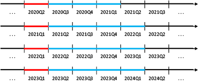
We define the dependent variable as a binary default indicator, which was calculated as follows. If the household was in default on its mortgage on 1 January of a given year, such a borrower was excluded for this year. If the borrower was not in default on its mortgage on the 01 January of a given year and then did not default during the year, the default indicator equals 0. Otherwise, if the borrower was not in default on its mortgage on 1 January of a given year and then defaulted during the year, the dependent variable equals 1. As a result, we obtained a dataset with only 6% of defaults, that is, highly unbalanced. This number corresponded to banks’ assessment of the probability of default on the given time horizon. Consequently, we used a maximum of four data points for each borrower (corresponding to default status in 2020, 2021, 2022, and 2023). The schematic representation of the construction process of the dependent variable is shown in Figure 1.
 – Gather performing (not in default) loans.
 – For each loan, check whether it becomes nonperforming (“1” if yes, “0” if no).
Borrower-specific variables were taken as of 1 January of the respective year. The macroeconomic variable was set to be equal to the actual GDP growth of the year. That is done to distinguish the effect of general macroeconomic conditions on all borrowers from individual metrics.
One of the most important metrics for credit risk models is a debt-service-to-income ratio (DSTI), which points out the ability of the borrower to serve their debt. The idea of DSTI inclusion is that borrowers with higher DSTI will default more often. In countries where DSTI is an active policy instrument, values around 40% are believed to be a limit after which the borrower may possess additional credit risk for banks. Following Nier et al. (2019), we got rid of DSTI values higher than 300%. The reason for such high DSTIs lies in the field of income confirmation. Banks in Ukraine do not pay much attention after loan issuance to income verification and updating. As long as the borrower pays on time, there is a chance that banks will not update data. The DSTI was calculated for each loan and then aggregated on the borrower level as a simple sum.
The borrower’s age is another crucial indicator that influences the probability of default. For example, in Slovakia, policy measures are different for different age groups. It is more difficult for elderly people to find the new job if needed. In Ukraine, mortgages are provided only if the person is under 60 years old as of the maturity date. That is why we expect that a higher age would contribute to a higher default probability.
One more popular variable in credit risk studies is income. Filatov and Kaminsky (2021) used the quadratic term of this variable. Interestingly, their results imply that after a certain critical point income contributes positively to default. They indicated that the reason for this result is that the data quality of the Ukrainian credit registry is low, and data points with high income cannot be fully trustworthy.
We also included the loan characteristics, such as residual maturity in years and interest rate. Nier et al. (2019) proved that residual maturity is a very powerful and robust predictor of default. They found that the more time is left to pay the loan, the higher the probability of default. Moreover, Doko et al (2021) found that both maturity and interest rate have high and significant information values for default prediction.
This study also incorporated credit risk metrics assessed by banks. Filatov and Kaminsky (2021) findings show that credit risk indicator based on Ukrainian Credit registry data has a hump-shaped impact on default probability.
Since all borrowers are influenced by general macroeconomic conditions, we incorporate the real GDP growth. We expect that the GDP growth is positively associated with the default probability: when the economic crises hit in 2020 and especially in 2022 in Ukraine, we observed higher default rates than in relatively calm 2021.
The final list of indicators for modelling and their descriptive statistics are presented in Table 1. The number of observations is 35828, with a unique number of borrowers equal to 18057. Annex A presents additional statistics for each variable.
The multicollinearity could be an issue for this ML study since we were interested in variable importance. From Table 2 we can conclude that no variables correlate much, and we can use them in the model.
|
Variable |
Level |
Unit of measurement |
Min |
Max |
Median |
Mean |
Proportion of zeros, % |
|
Annual income |
Borrower |
Thousand UAH |
0 |
320983 |
340 |
749 |
0 |
|
DSTI |
Borrower |
% |
0 |
300 |
22 |
34 |
2 |
|
Age |
Borrower |
Years |
21 |
72 |
39 |
40 |
0 |
|
Mortgage interest rate |
Loan |
% |
0 |
60 |
14 |
13,6 |
5 |
|
Aggregate borrower credit risk |
Borrower |
Thousand UAH |
0 |
23906 |
3,4 |
18,5 |
6 |
|
Residual maturity of mortgage |
Loan |
Years |
0 |
32 |
13,6 |
12,6 |
0,3 |
|
GDP growth |
Macroeconomy |
% |
-29,1 |
5,2 |
-3,45 |
-7,5 |
0 |
|
DSTI |
Age |
Credit risk |
Annual income |
Mortgage interest rate |
Residual maturity of mortgage |
GDP growth |
|
|
DSTI |
0,05 |
-0,0008 |
-0,09 |
0,11 |
-0,03 |
-0,12 |
|
|
Age |
0,05 |
0,02 |
0,0009 |
0,04 |
-0,37 |
0,005 |
|
|
Credit risk |
-0,0008 |
0,02 |
0,01 |
-0,07 |
0,002 |
0,01 |
|
|
Annual income |
-0,09 |
0,0009 |
0,01 |
0,0006 |
-0,01 |
0,01 |
|
|
Mortgage interest rate |
0,11 |
0,04 |
-0,07 |
0,0006 |
-0,08 |
0,03 |
|
|
Residual maturity of mortgage |
-0,03 |
-0,37 |
0,002 |
-0,01 |
-0,08 |
-0,01 |
|
|
GDP growth |
-0,12 |
0,005 |
0,01 |
0,01 |
0,03 |
-0,01 |
For classification tasks, the distribution of classes is crucial. As discussed above, our dataset is unbalanced, and it will be challenging for models to capture this nature. Moreover, it is more important for the bank to predict default in advance and act, rather than to believe that the borrower will continue to pay. There are two ways of handling the imbalance problem without changing the dataset: weight assignment and cost-sensitive learning. Setting efficient costs for type 1 and type 2 errors is an exercise that demands another research. The reason for that is that banks, after classifying the borrower as risky, are required to form reserves. For loans accounted on a group basis (most popular for mortgages) it means that reserves must be equal to 100% of the estimated risk, which is costly. That is why in this study, we used the weight assignment technique. To check the robustness of weighting, we also used the SMOTE algorithm, which is a popular method in credit risk studies.
The idea of weight assignment is that in the training phase of the model observations of different classes are assigned different weights. Since banks care more about default (the ones in our data), we assigned a higher weight to them. The advantage of this method is that it is simpler than other ones and does not change the sample. The disadvantage is the difficulty of assigning efficient weights that will maximize true positive values and minimize loss in overall accuracy. The weight of defaults was chosen to be inversely proportional to their number in the original dataset.
 (1)
(1)
where
wk – weight of unit in class k
nk – number of units in class k
Sample manipulation is a widespread group of methods in ML. One of the most popular methods that are used for credit risk modelling is SMOTE. It artificially creates an additional number of “defaults” and makes data balanced. The algorithm finds the difference between the given point and its nearest neighbour. This difference is multiplied by a random number in the interval from 0 to 1. The obtained value is added to the given point to form a new synthesized point in the feature space. Similar actions continue with the next nearest neighbour, up to the point when the sample will become balanced.
The classical classification methods are binary choice models, in particular a logistic regression (hereinafter logit). The main advantage of this model is its simplicity and easy interpretability. However, there are many disadvantages including linearity between dependent and independent variables and problems to work with datasets containing many features. That is why in this study we applied other methods as well. ML methods suggest new ways of separation between classes and as a result, provide high efficiency classification. The logit model would be the basis for comparison.
The models were chosen based on several papers that also studied credit risk. Doko et al. (2021) used logistic regression, decision trees, random forests, support vector machines, and neural networks. Kaminsky and Filatov (2021) applied XGBTree. Turkson et al. (2016) also applied linear discriminant analysis.
Linear Discriminant Analysis (LDA) is a statistical method aiming to find optimal linear combinations of features that maximize the separation between different classes. By projecting data onto a lower-dimensional space, LDA seeks to capture essential information while minimizing class overlap. Assumptions include multivariate normality and equal covariance across classes, rendering LDA effective when these assumptions hold. It is widely utilized in classification tasks where interpretability and dimensionality reduction are paramount (James et al., 2013).
Support Vector Machines (SVM) aim to find an optimal hyperplane that maximizes the distance (called margin) between different classes in feature space. SVM excels in high-dimensional spaces and can handle non-linear relationships through kernel functions. By focusing on the most critical data points, or support vectors, SVM delivers robust classification performance. For this research we used a linear model, leaving more complex ones for future studies. Mathematically, the optimization problem that is solved by this kind of model is given as follows (James et al., 2013):
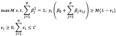 (4)
(4)
where
M – margin to optimize
ϵi – errors allowing observations to be on the wrong side of the plane
C – nonnegative tuning parameter
Classification and Regression Trees (CART) construct binary trees by recursively partitioning data based on feature splits. The algorithm optimizes impurity measures, such as the Gini index. CART’s simplicity, interpretability, and ability to handle both categorical and continuous data make it a versatile tool for classification tasks. For this method, it is especially crucial to make a trade-off between interpretability and accuracy. The more complex trees may produce better-classifying properties but are very difficult to understand.
Random Forest (RF), which is a more complicated version of CART, builds an ensemble of decision trees using bootstrap sampling and feature randomness. By aggregating predictions from multiple trees, it mitigates overfitting and enhances overall model accuracy. Random Forest excels in capturing complex relationships and interactions in diverse datasets. The significant plus of the RF models is that they overfit less than methods. The algorithm works by calculating the weighted Gini index and optimizing it to find the minimum one (Saini, 2022). For the binary data like in this study, the formula looks like this:
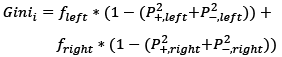 (2)
(2)
Where:
Ginii – Gini index at node i
fleft – fraction of values that went to the left on the split
fright – fraction of values that went to the right on the split
P+ – probability of getting positive class
P–– probability of getting negative class
XGBoost, an implementation of gradient boosting, focuses on maximizing computational efficiency and predictive accuracy. The XGBtree variant employs tree-based models, combining multiple weak learners to form a robust classifier. Through gradient boosting, XGBoost sequentially corrects errors of preceding models, showcasing superior performance in various domains. Its versatility, scalability, and adaptability to diverse datasets make XGBtree a popular choice for complex classification challenges. According to Beeravalli (2018), it is one of the most balanced methods for credit risk assessment. Filatov and Kaminsky (2021) also concluded that this method is applicable to credit risk assessment using Ukrainian data.
Comprising layers of interconnected artificial neurons, Neural Networks (NNET) leverage backpropagation to iteratively adjust weights, adapting to intricate patterns. Their capacity for hierarchical feature learning and representation makes them highly effective in capturing non-linear dependencies, making Neural Networks suitable for classification tasks where intricate relationships exist. The main definitions for Neural networks are weights and biases. Weights are coefficients that are multiplied by indicators. Bias is the constant that is added to the product of features and weights. The formulas for updating the network at each step are the following:
 (3)
(3)
where
wnew – new weight of variable i
wold – old weight of variable i
biasnew – new bias of variable i
biasold – old bias of variable i
learning rate – parameter that determines the size of the update step
One of the goals of this study was to assess which variables can be used as the best predictors for the default. This will be done through variable importance analysis. Since we used several ML methods, we should go through what is variable importance (VI) for each of them.
In Logit and LDA models, VI is based on the magnitude of the estimated coefficients. Larger coefficients suggest a stronger impact on the response variable. This method does not cause problems if we use linear models, however, adding interactions or polynomials may lead to “borrowing” importance between variables. In SVM models, coefficients are called “weights”, but the idea is the same: larger weights suggest a more important role in determining decision boundary.
In CART and RF models, VI is calculated based on the decrease of the Gini index at each split. The bigger in magnitude is the decrease in the Gini index, the more significant the variable is.
VI in XGBtree models provides a score that shows how useful a variable was in the construction of the tree. The more an attribute is used to make split decisions, the higher would be VI.
The VI analysis can also be applied to neural networks. We applied the methodology first proposed by Garson (1991). The basic idea is that the relative importance is calculated as a sum of all weighted connections between nodes that correspond to the variable of interest.
All variable importance scores were normalized in such a way that the most important variables would have a score value of 100, and the least important - 0. Where coefficients can have different signs (like in Logit or SVM), the absolute value was used for calculation.
To test the efficiency of each method, we split the data into training and testing sub-samples. There are no direct rules for the ratio of data split into training sets; however, standard practices use 70%/30%, 67%/33%, or 80%/20%. We chose the 70%/30% rule as the main one and other rules as robustness checks. We used the training sub-sample to estimate the parameters and the testing sub-sample to see the out-of-sample effectiveness. Cross-validation was included in the training phase with some folds equal to 100. Based on the test sample we calculated AUROCs and made a DeLong’s test for statistical difference between them. We followed the simple DeLong’s methodology as in DeLong et al. (1988). All variables have been scaled in a preprocessing stage, so the impact of different variables on the default outcome was comparable.
All models were compared via three dimensions. The first one is classification metrics such as accuracy, F-score, AUROC, and precision. The second dimension lies in the field of variable importance. There we concluded which variables play the most important role in default prediction. If the variable turned out to be important for several models, then it was robust to specifications, and we concluded that a change in that variable would lead to a change in default probability. Finally, we repeated this exercise for the weighted original sample and the sample after the SMOTE algorithm, to compare which method is more accurate for default prediction.
In this section, we presented the results for 7 ML models estimated on two datasets.
We started by analysing weighted original sample results. Figure 2 presents ROC curves with respective AUROC values. We observed that the logit model performed well both in terms of overall accuracy and precision of default prediction. However, it is worth mentioning that despite only 564 defaults in the test sample, the logit model predicted more than 3000. This result highlights the necessity to use more complex models because the model overshooted even though the data has been weighted there. The SVM and LDA models showed the worst results since they could not predict any defaults at all. Random Forest and XGBtree had significantly better performance in comparison to logit based on the AUROC metric and it was tempting to say that they would be the best for credit risk assessment.
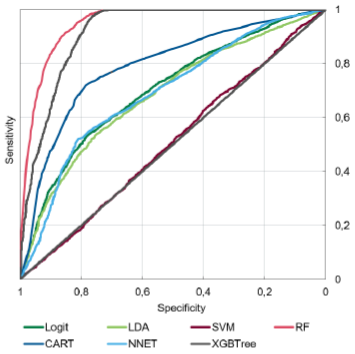
According to the results in Table 3, Models like Neural Net, CART, and logit due to a much higher number of predicted defaults in general, predicted a high number of correct defaults. However, since the correct number of defaults was only 564 it means, that usage of these models will predict thousands of excess defaults, which is also too risky for financial institutions. RF and XGBtree predict more correct defaults, with a lower number of false defaults. They do not overshoot with type 1 errors that much. These models provided the essential balance. It is also important to mention that all pairs of models except the NNET-LDA pair passed DeLong’s test for statistical difference between ROCs. From here, we conclude that RF and XGBtree showed the most accurate results based on predictive metrics not only in comparison to baseline logit but also among all presented models.
|
Model |
Logit |
LDA |
CART |
RF |
SVM |
NNET |
XGBtree |
|
Predicted number of 0 |
6990 |
10745 |
6377 |
8694 |
10747 |
6673 |
8973 |
|
Predicted number of 1 |
3757 |
2 |
4370 |
2053 |
0 |
4074 |
1774 |
|
Proportion of correct default prediction (precision), % |
67 |
0,2 |
77 |
92 |
0 |
72 |
96 |
|
F1 - score |
0,18 |
0,004 |
0,18 |
0,89 |
0 |
0,17 |
0,9 |
Table 4 presents results of variable importance. For the logit model GDP growth, credit risk, and age showed the biggest in magnitude impact on the probability of default. If we take a broader look at all models, it was quite expected that GDP growth would be a good predictor of default because in four models it turned out to be the most important one. However, in RF and XGBtree models it turned out the least important variable. The reason for that lies in the field of how VI is calculated for these models. Zero for tree-based models means that there are very few nodes in which GDP participates. The dataset includes only 4 years, so there is not enough variation for the model to make decisions based on macroeconomic conditions. Rolling window approach as well as gathering more data in the future is going to solve this problem.
According to the models’ results, DSTI also contributed a lot to default probability, especially in the XGBtree model (most important) and RF (second most important), which proved to be the best in the previous analysis step. It means that NBU can use it for its policy purposes. In contrast to similar studies, residual maturity did not play an important role in causing defaults. This means that banks’ monitoring policy should treat equally borrowers with high residual maturity as well as those who nearly repaid the debt.
As an interim summary, we could say that RF and XGBtree models suit better than Logit to estimate the default probability on a one-year horizon. They perform well in terms of overall accuracy and precision in insolvency prediction. The results of models slightly contradict which variables contribute more to the default probability, so let’s see how SMOTE estimations performed.
|
Variable |
Logit |
LDA |
CART |
RF |
SVM |
NNET |
XGBtree |
|
DSTI |
10,31 |
25,07 |
25,92 |
83,18 |
25,07 |
0 |
100 |
|
Income |
8,66 |
30,08 |
32,26 |
81,90 |
30,08 |
0,06 |
93,74 |
|
Age |
29,03 |
28,27 |
35,97 |
81,35 |
28,27 |
29,01 |
87,05 |
|
Interest rate |
20,82 |
30,79 |
36,01 |
53,97 |
30,79 |
31,01 |
76,75 |
|
Credit risk |
49,24 |
69,89 |
100 |
100 |
69,89 |
44,32 |
65,69 |
|
Residual maturity |
0 |
0 |
20,9 |
67,78 |
0 |
28,51 |
55,88 |
|
GDP growth |
100 |
100 |
0 |
0 |
100 |
100 |
0 |
According to Figure 3, the ROCs looked nearly the same as on the unbalanced sample, except for the LDA model. DeLong’s test for the difference between AUROCs failed for LDA-SVM pairs, which is interpreted as that their overall accuracy was very close.
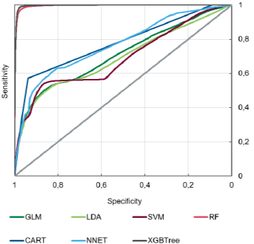
However, when we checked the precision (Table 5), we observed that all models except for RF and XGBtree again overshoot with the total number of defaults. Moreover, even though RF and XGBtree predicted fewer defaults than other models, they predicted more defaults that were correct this time, which is especially crucial for banks. Because SMOTE made the sample balanced, the precision of all models increased.
|
Model |
Logit |
LDA |
CART |
RF |
SVM |
NNET |
XGBtree |
|
Predicted number of 0 |
9935 |
10305 |
8896 |
10390 |
10196 |
10335 |
10415 |
|
Predicted number of 1 |
10416 |
10046 |
11455 |
9961 |
10155 |
10016 |
9936 |
|
Proportion of correct default prediction (precision), % |
70 |
66 |
80 |
90 |
67 |
77 |
92 |
|
F1-score |
0,68 |
0,66 |
0,76 |
0,91 |
0,67 |
0,77 |
0,93 |
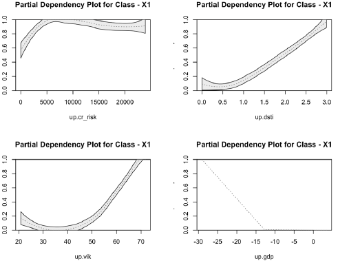
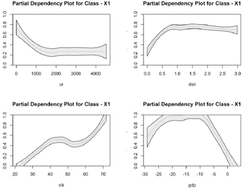
Now let us check which variables contribute to the default probability on the balanced synthesized data. Models on these data were not much different from the previous ones. GDP growth, Credit risk, and DSTI variables turned out to be the best predictors. Surprisingly XGBtree and RF models that showed the best results on the weighted original sample, revealed contradictive results after SMOTE. While XGBtree was in line with its previous conclusion that DSTI was the most important variable, the RF model showed that it was among the least important ones. That is also counterintuitive because for the RF model partial dependency of default outcome on DSTI was high on both original data and SMOTE, which is illustrated in Annex B. The reason for that is that in this kind of model, importance means taking part in splitting trees. Partial dependence, on the contrary, shows how changing the predictor by 1 unit will change the probability of the outcome. Therefore, even though there are not many nodes where DSTI took part in the decision, it is still significant in general.
|
Variable |
Logit |
LDA |
CART |
RF |
SVM |
NNET |
XGBtree |
|
DSTI |
9,75 |
47,31 |
11,96 |
2,79 |
47,31 |
58,67 |
100 |
|
Income |
0 |
14,7 |
0 |
2,22 |
14,7 |
0 |
60,28 |
|
Age |
28,61 |
28,42 |
0,99 |
0 |
28,42 |
38,02 |
45,15 |
|
Interest rate |
19,44 |
31,26 |
14,05 |
20,08 |
31,26 |
61,65 |
38,93 |
|
Credit risk |
49,15 |
100 |
35,13 |
8,39 |
100 |
26 |
14,23 |
|
Residual maturity |
1,84 |
0 |
9,1 |
10,16 |
0 |
57,17 |
13,52 |
|
GDP growth |
100 |
79,26 |
100 |
100 |
79,26 |
100 |
0 |
Annex C presents the robustness checks based on other train-test splittings, namely, 80%/20% and 67%/33%. We compared the overall performance of the models and concluded that the results are not much different for both weighting and SMOTE-synthesized datasets, which means that the current specification is robust. XGBtree model still shows the best accuracy and precision results.
In this study, we examined how Credit registry data can predict the default of borrowers with mortgages using machine learning techniques.
First, we showed that Random Forest and XGBtree models were the most suitable for insolvency prediction among ML modelling techniques and showed better performance than logistic regression. They provided the essential balance between correct default classification and minimizing false defaults. These models showed robust results and predicted defaults most efficiently on both weighted data and SMOTE-synthesized.
Second, GDP growth and DSTI turned out to be the best predictors of mortgage default on a one-year horizon independent of the data sample and its transformations. This result is useful for both banks and policymakers. On one hand, it means that banks in general adequately measure credit risk, and on a one-year horizon borrowers become insolvent if the risk increases. On the other hand, DSTI is an effective policy instrument that can mitigate risk accumulation. For example, the National Bank may introduce new capital measures for borrowers with high DSTI. Furthermore, adequate GDP forecasting can lead to increased accuracy in default probability.
Third, the study explored data balancing techniques. The findings are that models estimated on the SMOTE sample showed better performance than those on data weighted sample. In further studies, the authors will investigate other balancing techniques.
As policy recommendations for the regulator, we suggest that NBU may accelerate with DSTI introduction as a macroprudential instrument. This could potentially decrease the number of defaults in the future. As to recommendations for commercial banks, they should pay close attention to all borrowers irrespective of their loan maturities. It is essential for them to direct their focus to income verification because it is the key to correct DSTI calculation. Using DSTI as a proper instrument could help NBU monitor the systemic risk in household lending, while commercial banks will do provisioning on time.
Further borrower insolvency studies can help banks detect the realisation of credit risk in advance and take action. Machine learning will play a key role here since traditional logistic regression is limited in its capabilities to capture complex relations. ML methods can maximize the accuracy of forecasting, at the same time minimizing false default predictions. Moreover, machine learning models can offer insights into patterns within the data that traditional methods might overlook. Incorporating in future collateral characteristics in the study may also provide insights not only into the PD estimation but also its relationship with a loss given default, which is still a question for Ukrainian banks. ML methods can explain this relationship better than traditional linear or logistics models.
The dataset used in this research used the period of 2020–2023. As a further extension, the authors will broaden the horizon to 2024. Further studies will also include testing other time periods like 2021–2023 or 2021–2022. This could potentially lead to other factors playing a role, which in turn can change the predictive power of the model.
Bakırarar, Batuhan and Atilla Elhan. 2023. “Class Weighting Technique to Deal with Imbalanced Class Problem in Machine Learning: Methodological Research.” Turkiye Klinikleri Journal of Biostatistics. 15. 19-29. https://doi.org/10.5336/biostatic.2022-93961.
Bank of England, Financial Conduct Authority. 2022. “Machine learning in UK financial services.”
Batista, Gustavo, Ronaldo Prati, and Monard, Maria-Carolina. 2004. “A Study of the Behavior of Several Methods for Balancing machine Learning Training Data”. SIGKDD Explorations. 6. 20-29. https://doi.org/10.1145/1007730.1007735.
Beeravalli, V. 2018. “Comparison of Machine Learning Classification Models for Credit Card Default Data.” Retrieved from https://medium. com/@vijaya.beeravalli/comparison-of-machine-learning-clas- sification-models-for-credit-card-default-data-c3cf805c9a5a.
Buzanov Gleb and Andrey Shevelev. 2022. «Probability of default model with transactional data of Russian companies.» IFC Bulletins chapters, in: Bank for International Settlements (ed.), Machine learning in central banking, volume 57, Bank for International Settlements.
Costa, André Faria da, Fonseca, Francisco and Maurício, Susana. 2022. “Novel methodologies for data quality management Anomaly detection in the Portuguese central credit register in Settlements”, Bank for International eds., Machine learning in central banking, vol. 57, Bank for International Settlements, https://EconPapers.repec.org/RePEc:bis:bisifc:57-29.
Datsyuk Yuliya. 2024. “7 Top Machine Learning Use Cases in Banking and Financial Industry.” Retrieved from https://kindgeek.com/blog/post/5-top-machine-learning-use-cases-in-finance-and-banking-industry#:~:text=ML%20algorithms%20are%20employed%20for,transaction%20behaviour%20for%20further%20investigation.
DeLong, Elizabeth R., David M. DeLong, and Daniel L. Clarke-Pearson. 1988. “Comparing the Areas under Two or More Correlated Receiver Operating Characteristic Curves: A Nonparametric Approach.” Biometrics 44, no. 3 : 837–45. https://doi.org/10.2307/2531595.
Dumitrescu Elena, Sullivan Hué, Christophe Hurlin and Sessi Tokpavi, 2022. “Machine learning for credit scoring: Improving logistic regression with non-linear decision-tree effects.” European Journal of Operational Research, Volume 297, Issue 3. https://doi.org/10.1016/j.ejor.2021.06.053.
Dirma, Mantas and Jaunius Karmelavičius. 2023. “Micro-assessment of macroprudential borrower-based measures in Lithuania”. Bank of Lithuania Occasional Paper Series 46/2023.
Doko, Fisnik, Slobodan Kalajdziski, and Igor Mishkovski. 2021. “Credit Risk Model Based on Central Bank Credit Registry Data.” Journal of Risk and Financial Management 14, no. 3: 138. https://doi.org/10.3390/jrfm14030138
Filatov, Vladyslav, and Аndriy Kaminsky. 2021. “Application of the Scoring Approach to Monitoring Function of Central Bank Credit Registry”. Scientific Papers NaUKMA. Economics, 6(1), 73–83. https://doi.org/10.18523/2519-4739.2021.6.1.73-83
Garson, G.D. 1991. “Interpreting neural-network connection weights.” AI Expert 6(4): 46-51. https://dl.acm.org/doi/abs/10.5555/129449.129452
Gupta Palak, Anmol Varshney, Mohammad Rafeek Khan, Rafeeq Ahmed, Mohammed Shuaib, Shadab Alam. 2023. “Unbalanced Credit Card Fraud Detection Data: A Machine Learning-Oriented Comparative Study of Balancing Techniques.” Procedia Computer Science, Volume 218 https://doi.org/10.1016/j.procs.2023.01.231.
James, Gareth, Daniela Witten, Trevor Hastie, and Robert Tibshirani. 2013. “An Introduction to Statistical Learning”. PDF. 1st ed. Springer Texts in Statistics. New York, NY: Springer.
Liashenko, Olena, Kravets, Tetyana and Kostovetskyi, Yevhenii. 2023. “Machine Learning and Data Balancing Methods for Bankruptcy Prediction.” Ekonomika, 102(2), pp. 28–46. doi:10.15388/.
Li, Peng & Rao, Susie, Blase, Jennifer, Zhang, Yue, Chu, Xu and Zhang, Ce. 2021. “CleanML: A Study for Evaluating the Impact of Data Cleaning on ML Classification Tasks”. In: Proceedings of the International Conference on Data Engineering (ICDE), pp. 13–24.
Nier, Erlend, Radu Popa, Maral Shamloo, and Liviu Voinea. 2019. “Debt Service and Default: Calibrating Macroprudential Policy Using Micro Data.” IMF Working Papers, 182, A001. https://doi.org/10.5089/9781513509099.001.A001
Regulation No. 351 dated 30 June 2016 “On Measuring Credit Risk Arising from Banks’ Exposures.” Retrieved from https://zakon.rada.gov.ua/laws/show/v0351500-16#Text
Saini, Anshul. 2022. “An Introduction to Random Forest Algorithm for beginners”. Retrieved from https://www.analyticsvidhya.com/blog/2021/10/an-introduction-to-random-forest-algorithm-for-beginners/
Shen, Feng, Xingchao Zhao, Zhiyong Li, Ke Li, Zhiyi Meng. 2019. “A Novel Ensemble Classification Model Based on Neural Networks and a Classifier Optimisation Technique for Imbalanced Credit Risk Evaluation.” Physica A: Statistical Mechanics and Its Applications, 526, Article ID: 121073. https://doi.org/10.1016/j.physa.2019.121073
Turkson, Regina Esi, Edward Yeallakuor Baagyere, and Gideon Evans Wenya. 2016. “A Machine Learning Approach for Predicting Bank Credit Worthiness.” Paper presented at the 2016 Third International Conference on Artificial Intelligence and Pattern Recognition (AIPR), Lodz, Poland, September 19–21; Piscataway: IEEE, pp. 1–7.
Xu, Ziyu, Chen Dan, Justin Khim, and Pradeep Ravikumar. 2020. “Class-Weighted Classification: Trade-offs and Robust Approaches.” ArXiv abs/2005.12914
|
Variable |
Skewness |
Kurtosis |
|
Annual income |
1,5 |
1,89 |
|
DSTI |
1,14 |
1 |
|
Age |
0,54 |
0,06 |
|
Mortgage interest rate |
-0,09 |
2 |
|
Aggregate borrower credit risk |
2,08 |
4,3 |
|
Residual maturity of mortgage |
-0,15 |
-1,05 |
|
GDP growth |
-0,66 |
-1,44 |
|
Model |
Logit |
LDA |
CART |
RF |
SVM |
NNET |
XGBtree |
|
Predicted number of 0 |
4618 |
7163 |
4830 |
5773 |
7165 |
4439 |
5598 |
|
Predicted number of 1 |
2547 |
2 |
2335 |
1392 |
0 |
2726 |
1567 |
|
Proportion of correct default prediction (precision), % |
70 |
0,003 |
69 |
96 |
0 |
75 |
97 |
|
F1 - score |
0,18 |
0,005 |
0,19 |
0,88 |
0 |
0,18 |
0,88 |
Weighted sample model results on 66%/33% split
|
Model |
Logit |
LDA |
CART |
RF |
SVM |
NNET |
XGBtree |
|
Predicted number of 0 |
7772 |
11939 |
7156 |
9701 |
11942 |
7379 |
10280 |
|
Predicted number of 1 |
4170 |
3 |
4786 |
2241 |
0 |
4563 |
1662 |
|
Proportion of correct default prediction (precision), % |
66 |
0,003 |
78 |
96 |
0 |
73 |
94 |
|
F1 - score |
0,17 |
0,006 |
0,18 |
0,89 |
0 |
0,18 |
0,90 |
SMOTE-synthesized sample model results on 80%/20% split
|
Model |
Logit |
LDA |
CART |
RF |
SVM |
NNET |
XGBtree |
|
Predicted number of 0 |
6565 |
6868 |
5906 |
6859 |
6742 |
6914 |
6839 |
|
Predicted number of 1 |
7002 |
6699 |
7661 |
6708 |
6825 |
6653 |
6728 |
|
Proportion of correct default prediction (precision), % |
70 |
66 |
75 |
97 |
67 |
78 |
98 |
|
F1 - score |
0,69 |
0,66 |
0,75 |
0,97 |
0,67 |
0,78 |
0,98 |
SMOTE-synthesized sample model results on 66%/33% split
|
Model |
Logit |
LDA |
CART |
RF |
SVM |
NNET |
XGBtree |
|
Predicted number of 0 |
11032 |
11486 |
9930 |
11397 |
11309 |
11561 |
11403 |
|
Predicted number of 1 |
11581 |
11127 |
12683 |
11216 |
11304 |
11052 |
11210 |
|
Proportion of correct default prediction (precision), % |
69 |
66 |
80 |
97 |
68 |
77 |
97 |
|
F1 - score |
0,69 |
0,67 |
0,76 |
0,97 |
0,68 |
0,78 |
0,98 |