Ekonomika ISSN 1392-1258 eISSN 2424-6166

2024, vol. 103(2), pp. 90–108 DOI: https://doi.org/10.15388/Ekon.2024.103.2.5

Modelling the Relationship Between Public Expenditure, Tax Revenue and Economic Growth in Türkiye Using the AARDL Approach

Ahmet Köstekçi
Fırat University, Elaziğ, Turkey
Email: akostekci@firat.edu.tr
ORCID: https://orcid.org/0000-0001-8485-887X

Ali Celik*
Istanbul Gelisim University, Istanbul, Turkey
Western Caspian University in Baku, Azerbaijan
Email: alcelik@gelisim.edu.tr
ORCID: https://orcid.org/0000-0003-3794-7786

Abstract. This study aims to investigate the macroeconomic impact of fiscal policy in Türkiye, where fiscal policy faces several challenges. Using annual time series data from 1980 to 2021, we examine the impact of tax and public expenditure subcomponents on GDP using the augmented autoregressive distributed lag (A-ARDL) bound test approach proposed by Sam et al. (2019). The A-ARDL test results indicate that tax revenue has a positive impact on economic growth in the short run, while tax revenue has a negative impact on economic growth in the long run. Furthermore, we conclude that increases in current and investment expenditures have a positive impact on economic growth in the short and long run, while increases in transfer expenditures have a negative impact on economic growth in the short run.
Keywords: Fiscal policy, Tax revenue, Public expenditure, Economic growth, Türkiye

_______

* Correspondent author.

Received: 16/02/2024. Revised: 09/04/2024. Accepted: 29/04/2024
Copyright © 2024 Ahmet Köstekçi, Ali Celik. Published by Vilnius University Press
This is an Open Access article distributed under the terms of the Creative Commons Attribution License, which permits unrestricted use, distribution, and reproduction in any medium, provided the original author and source are credited.

1. Introduction

Historically, there have been periods when the importance of fiscal policy as a policy instrument has increased or decreased. For example, with the stock market crash and the Great Depression, policymakers pushed for a more active role of the state in the economy (Horton & El-Ganainy, 2019). As a result, market failures allowed for the implementation of fiscal policy, which was Keynes’s primary tool for the interventionist economic approach. However, after the 1970 oil crisis, both advanced and emerging economies faced the problem of fiscal imbalances and the debt-to-GDP ratio rose above 100 percent in some countries that financed their budget deficits by borrowing (Karagöz & Keskin, 2016, p. 409). This large fiscal shock forced policymakers to answer various questions about how to solve the problems. During this period, when the concept of government failure began to be scrutinized in academic circles (Buchanan, 1983; Krueger, 1990), a negative perspective on the implementation of fiscal policy emerged. The negative view of fiscal policy was not limited to the 1970s, but continued until the early 2000s (Dullien, 2012, p. 7).

Despite these changes, which reduced the role and influence of government in the economy, many countries resumed more active fiscal policies when the global financial crisis threatened a global recession (Horton & El-Ganainy, 2019). For instance, during the economic crisis of 2008, governments intervened to support financial systems, stimulate economic growth, and mitigate the impact of the crisis on vulnerable populations. This made the role and objectives of fiscal policy particularly important. Indeed, in the statement following their April 2009 summit in London, G20 leaders declared that they had embarked on an unprecedented and coordinated fiscal expansion (Horton & El-Ganainy, 2019). As fiscal stimulus expanded and was on the agenda of all countries, it was debated whether tax cuts or spending increases would be a better solution for these countries (Alesina & Ardagna, 2009).

After the 2008 crisis, the expansion of fiscal stimulus was supported not only by national and international monetary and fiscal authorities but also by economists. Indeed, the results of the policies implemented confirmed the effectiveness of fiscal policy in stabilizing aggregate demand, especially during periods of extraordinary economic weakness (Dullien, 2012). Similarly, the changes in fiscal policy due to the coronavirus pandemic (COVID-19), which started in 2019, were notable (Weinstock, 2021). In response to pandemics that have historically caused severe recessions, many countries and policymakers have resorted to active fiscal policies or offered various fiscal policy packages (Afonso & Coelho, 2023; Boug et al., 2023; Chudik et al., 2021). As a result, even if the fiscal consolidation approach is insufficient, fiscal policy has been reinvigorated in the global discourse over the last quarter century (Woldu & Kano, 2023) and finding an effective fiscal policy mix is more important today than ever (Donadelli & Grüning, 2021). In this subject, information on the economic effects of fiscal policy is an important element to guide the achievement of fiscal sustainability and should be taken into account in the design and recommendation of public policies (Sosvilla-Rivero & Rubio-Guerrero, 2022). Therefore, in this study, which aims to examine the effects of tax and expenditure policies, we consider Türkiye as an interesting and important example. This is because Türkiye, which struggled with high budget deficits in the 1990s, managed to create a strong fiscal structure by ensuring fiscal discipline in the early 2000s. However, due to the policies implemented in recent years, fiscal policy in Türkiye has faced various challenges and the macroeconomic effects of fiscal policy have become an important topic of debate.

Our main hypothesis is that fiscal policy has a significant effect on GDP growth in Türkiye, but this effect differs significantly across the subcomponents of fiscal policy instruments. Within the scope of this hypothesis, the main motivation and objective of this study is to empirically determine whether fiscal policy is effective in stimulating economic activity in Türkiye and, if so, the strength and duration of these effects. In this sense, specific questions such as whether the subcomponents of fiscal policy instruments have different effects in promoting economic growth and which of the subcomponents of fiscal policy instruments have stronger effects on economic growth constitute the research questions of our study. The answers to these questions will contribute to the ongoing debate on the role of fiscal policy. Based on the basic information provided, the sections of the study after the introduction are organized as follows. The empirical literature related to previous studies is presented in Section 2. The data set, model and methodology are indicated in Section 3. Section 4 presents the empirical results. The paper ends with conclusions and policy recommendations.

2. Literature Review

Fiscal policy, in which governments can influence economic activity by using public expenditures, tax revenues or both (Alves & Palma, 2023; Karaş & Karaş, 2023; Weinstock, 2021), has recently attracted attention. This is particularly evident during economic cycles (Caldara & Kamps, 2017; Ramey & Zubairi, 2018; Terra et al., 2021). On the other hand, regardless of business cycles, many countries resort to contractionary fiscal policy measures to reduce public debt levels that increase as a result of fiscal expansion (Alesina & Ardagna, 2009; Alesina et al., 2015; Arizala et al., 2021; Christelis et al., 2019; Rompuy, 2021; Woldu & Kano, 2023). Despite the role of fiscal policy, there is no consensus on the size and effectiveness of the subcomponents of fiscal instruments and there is still debate on the implementation of fiscal policy from a macroeconomic perspective (Fukuda, 2023; Gootjes & Haan, 2022; Heimberger, 2023; Mawejjeve & Odhiambo, 2022).

The impact of fiscal policy is assessed by Blanchard and Perotti (2002) using data on the elasticity of fiscal variables. They conclude that expansionary fiscal shocks boost output, have positive effects on private consumption, and negatively affect private investment. Castro (2006), who analyzed the macroeconomic effects of fiscal policy in Spain with data for the period 1980–2001, concluded that increases in public expenditures have a positive effect on GDP in the short run. However, this effect was found to be negative in the medium and long run. Pointing to the non-Keynesian effects of fiscal policy, the article showed that a fiscal consolidation based on expenditure cuts can have an expansionary effect on economic activity. Giordano et al. (2007) found in a related study that public spending has a positive and long-term impact on output in Italy. The SVAR method is used by Mountford and Uhlig (2009) to analyze the effects of fiscal policy in the United States using quarterly data covering the years 1955–2000. According to the study’s primary findings, tax cuts financed by deficits are the best fiscal policy for improving GDP and stimulating the economy. However, this research illustrates the neoclassical view of government intervention in the economy because of the long-term costs of fiscal expansion with public expenditures. Conversely, Jawaid et al. (2010) find that the Keynesian perspective is reflected in these effects and that fiscal policy is a crucial macroeconomic policy tool for supporting output growth in Pakistan.

Parkyn and Vehbi (2014) examine the impact of public expenditure and revenue on output in New Zealand. They find that public expenditure shocks have a small positive effect on output in the short run but lead to lower output in the medium and long run. Although the effect of changes in tax revenue on GDP is less pronounced, it is found to be moderate. Therefore, the researchers found that the impact of discretionary fiscal policy on GDP is pro-cyclical. Using data from 1970 to 2009 for 20 OECD countries, Yang et al. (2015) conclude that short-term fiscal adjustments always have a contractionary effect on economic activity. Regarding the function of the composition of the fiscal adjustment, they find that output reductions from expenditure-based fiscal adjustments are smaller than those from tax-based fiscal adjustments. However, theoretical models suggest that households’ marginal propensity to consume may sometimes have binding borrowing constraints and may be asymmetric in the face of temporary changes in income or expenditure (Sosvilla-Rivero & Rubio-Guerrero, 2022). In this context, Bunn et al. (2018) find that households’ marginal propensity to consume is higher under negative income shocks than under positive shocks. This implies that a large part of the expenditure asymmetry can be explained by households’ balance sheet characteristics such as high debt levels, small liquidity buffers, concerns about the credit, and the possibility of low future income.

Pula and Elshani (2018) for Kosovo economy and Arin et al. (2019) for OECD countries conducted similar studies and found results supporting the Keynesian view. In another study, Afonso and Aubyn (2019) examined the macroeconomic impact of public and private investment spending based on data from 17 OECD countries in 1960–2014, using VAR analysis. Using impulse response functions, the researchers found that public investment spending has a contractionary effect in Finland, the UK, Sweden, Japan, and Canada, and a positive effect in most other countries. The study also found empirical evidence that public investment spending crowds out private investment spending. In terms of expenditures, current spending boosts economic growth, according to the findings of the Selvanathan et al. (2021) study. In contrast to this study, Onifade et al. (2020) find that current expenditures have strong and opposite effects on economic growth.

Sosvilla-Rivero and Rubio-Guerrero (2022) examined the short- and long-term symmetric and asymmetric effects of fiscal policy on output. Using quarterly data from 1980 to 2020, they find that while reductions in public spending or increases in net incomes reduce the short- and long-term effects on growth, increases in public spending and decreases in net incomes contribute to Spain’s economic growth in the short and long run. Golpe et al. (2023), in their study with quarterly data for the period 1990–2019 for 12 EU countries, found that monetary policy plays a leading role in economic growth in the complex economic system, while aggregate public expenditures are an important instrument supporting the driving force of fiscal policy. Amri et al. (2023) used a panel data set of 24 Indonesian provinces from 2006 to 2015 to apply a dynamic GMM model to estimate the effect of public expenditure on growth. The researchers found evidence that public spending significantly boosts economic growth. However, it turned out that local tax efforts had a negative impact on growth in the economy. However, the results of the study conducted by Alves and Palma (2023) with the Mixed Frequency Vector Autoregressive (MIDAS-VAR) model for Brazil showed that public expenditures have no significant effect on real GDP growth.

Turning to the case of Türkiye, there have been many studies on the relationship between fiscal policy and GDP growth. However, the limited number of studies with subindicators of fiscal policy instruments suggests that more studies are needed for more specific results. Using data for Türkiye from 1998 to 2016, Karahan and Çolak (2019) show that public spending has a positive impact on economic growth in the short run and a negative impact in the long run. From an economic policy perspective, there is significant evidence that expansionary fiscal policy can support economic growth in the short run. Arteris et al. (2021) conducted a different study and analyzed the comparative effectiveness of monetary and fiscal policy for Türkiye. Although both fiscal and monetary policies can affect output growth to different degrees, empirical evidence suggests that monetary policy has a greater impact on output growth. The results on fiscal policy show that direct and indirect taxes negatively effect output growth in the short and long term, while public consumption and investment expenditures have a positive effect on output. Özer and Karagöl (2018) analyzed the effect of monetary and fiscal policies on growth in the Turkish economy for the period 1998–2016 and found that monetary policy has only a short-term effect on growth, while fiscal policy affects growth in the long run and causes growth. Duran (2022), using the ARDL bounds test for the period 1975–2020, finds that the effect of subcomponents of public expenditure on economic growth in Türkiye is positive. In summary, it is noted that there is disagreement in Türkiye’s empirical literature on the topic.

3. Data set, model and methodology

3.1. Data and model

The study examines the effects of fiscal policy in Türkiye over the period 1980–2021. Accordingly, Table 1 shows the variables used in the study and the sources from which the data were compiled. The econometric model used in the study is based on the Keynesian expenditure model. John Maynard Keynes created a simplified version of the economy known as the Keynesian Expenditure Model or Aggregate Expenditure Model. The main focus of this model is the relationship between the level of aggregate expenditure and the level of real GDP. In an open economy, consumption (C), investment (I), government spending (G), and net exports (NX) are the basic expenditure components in the model (Keynes, 1936). The sum of government spending, net exports, investment, and consumption is the final planned total expenditure in the economy. When planned total expenditures (AE) and total income (Y) are equal, macroeconomic equilibrium is reached. In this case, for the equilibrium condition:

AE = Y = (C₀ + c(Y – T)) + I₀ + G₀ + (X − M) (1)

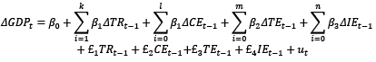
In summary, the equilibrium level of real GDP in the Keynesian Expenditure Model is represented by this equation. It indicates that the equilibrium GDP is determined by autonomous consumption (C₀), marginal consumption propensity (C), autonomous investment (I₀), autonomous government spending (G₀), taxes (T), and net exports (NX). This means that a change in taxes or autonomous expenditures (like government spending, investment, etc.) will result in a change in national income. In this theoretical framework, we generate our econometric model in which the net export variable is not utilized as follows:

GDP_t = α₀ + α₁TR_t + α₂CE_t + α₃IE_t + α₄TE_t + u_t (2)

In Eq. (2), the subscript states the time period. In addition, α₀ shows a constant term, while u_t refers to the error term. In addition, we employed Gross Domestic Product (GDP) as the dependent variable, while using Tax Revenues (TR), Current Expenditure (CE), Investment Expenditure (IE), and Transfer Expenditure (TE) as independent variables.

Table 1. The description of variables

3.2. Methodology

3.2.1. Unit root test

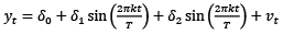
As is known, traditional unit root tests such as Augmented Dickey–Fuller (ADF) (1979) and Phillips–Perron (PP) (1989) are linear traditional unit root tests that do not take into account structural breaks. The Fourier ADF test developed by Christopoulos and Leon Ledesman (2010), which can be considered one of the current unit root tests modelling structural breaks in series with trigonometric terms, was used. The main advantage of this test is that it allows for smooth transitions as well as structural changes. Fourier ADF test statistics are calculated as follows (Christopoulos & Leon-Ledesman, 2010):

(3)

Here, k denotes the frequency number of the Fourier function, t denotes the trend, and T states the number of observations. The test statistic is calculated in three steps.

In the first stage, the appropriate frequency k* is determined. Thus, the nonlinear deterministic component in the above model will be determined by choosing the optimal k among k values between 1 and 5, which will be the value that minimizes the residual sum of squares through the least squares estimator.

(4)

In the second stage, the least squares residuals in the first stage are tested for unit root. Three separate models with the following linear and nonlinear structure are proposed:

(5)

(6)

(7)

Here θ>0 and u_t represents the error term. If the null hypothesis stating the existence of a unit root is rejected in the second stage, that is, if the series is stationary, the third stage is started. If the null hypothesis is rejected, it is concluded that the series is stationary around the structural deterministic function (Christopoulos & Leon-Ledesman, 2010).

3.2.2. Augmented ARDL method

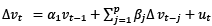
ARDL cointegration test, unlike traditional cointegration tests, provides analysis for variables with different degrees of stationarity (Pesaran & Shin, 1995; Pesaran et al., 2001). The ARDL test requires that the dependent variable I(1) and the independent variables I(0) or I(1) be stationary (Pesaran et al., 2001). However, the augmented ARDL (A-ARDL) method introduced by Sam et al. (2019) does not require the dependent variable to be stationary at I(1). To implement the ARDL model in cases where the dependent variable is stationary, McNown et al. (2018) and Sam et al. (2019) introduced a new F-test for lagged independent variables. Therefore, it can be utilized especially when the dependent variable is stationary at I(0) (Sam et al., 2019). Three tests (F bounds test statistics, t bounds test statistics, the Exogenous F-Bound) are employed for A-ARDL method. When these three tests are statistically significant together, there is a cointegration relationship between the variables. We established the ARDL model as follows.

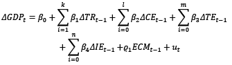
(8)

In Eq. (8), a₀ denotes the constant term, while Δ denotes the difference operator, and u_t indicates the error term, respectively. k, l, m, and n terms denote optimal lag length. The null and alternative hypotheses regarding the ARDL bounds test are presented below.

H₀: £₁ = £₂ = £₃ = £₄ = 0 (No cointegration relationships existed between variables)

H₁: £₁ = £₂ = £₃ = £₄ ≠ 0 (Cointegration relationships existed between variables)

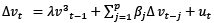
In Eq. (8), £₁, £₂, £₃, £₄ denote the long-run paramaters. However, in Eq. (9), the short-run and error correction model (ECM) is given below:

(9)

In Eq. (9), β₁, β₂, β₃, and β₄ state the short-run parameters, while ECM_t–1 denotes the error correction term with a lagged, and ϱ₁ denotes the error correction paramater. The fact that the coefficient of ECM_t–1 is statistically significant and has a negative sign means that any long-run disequilibrium between the dependent variable and a set of independent variables will converge back to the long-run equilibrium association.

4. Empirical results

Table 2 provides the statistical values of the variables used in the study. It appears that the mean of GDP is 4.59%, the mean of TR is 13.43%, the mean of CE is 7.23%, the mean of TE is 10.99% and the mean of IE is 1.78%. On the other hand, the median of GDP is 5.03%, the median of TR is 14.93%, the median of CE is 7.72%, the median of TE is 11.50%, and the median of IE is 1.67%. In addition, the maximum value of GDP is 11.35%, while the minimum value of GDP is -5.75%. The maximum value for TR is 18.01%, while the minimum value for TR is 7.85%. The maximum value of CE is 8.83%, while the minimum value of CE is 4.33%. The maximum value of TE is 22.80%, while the minimum value of TE is 3.79%. The maximum value of IE is 2.81%, while the minimum value of TR is 0.85%. The JB normality distribution results of the variables reveal that the variables have a normal distribution except for the TR and CE variables.

Table 2. Descriptive Statistics of tha data

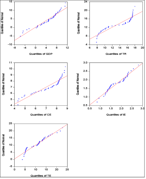
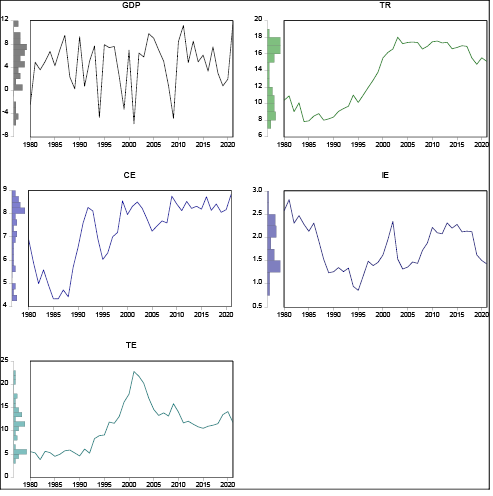
The quantile distributions of the variables in Figure 1 also indicate that there is no difference in the geometric scale of the variable distributions. Therefore, the series are used in their raw form and a linear model is fitted. Figure 2 also presents a graphical view of the variables.

Figure 1.

Figure 2. Graphical view of variables

4.1. Unit root test findings

In this study, traditional unit root tests (ADF and PP) were first used to measure the level of stationarity of the series. According to this, as seen in Table 3, the null hypothesis is rejected for both the constant model and the constant and trend model for the dependent variable used. In other words, GDP is stationary at the level values of the variable. Table 3 indicates that the independent variable CE is stationary at level values for the model with trend and constant. Apart from this, the other independent variables became stationary after taking the first difference for both the model with constant and the model with constant and trend. In summary, our dependent variable is stationary at I(0) and our independent variables are stationary at I(0) and I(I). Moreover, ADF and PP unit root test results are consistent with our Fourier ADF unit root test results indicated in Table 4. In line with these test results, it is appropriate to apply the A-ARDL test method proposed by Sam et al. (2019) in the advanced stages of our study.

Table 3. ADF and PP unit root test results

Note. *, **, and *** denote the significance level at the 10%, 5%, and 1%, respectively.

Table 4. Fourier ADF unit root test results

Note. *** denotes the significance level at the 10%. For critical values, we referred to the work of Christopoulos and Leon-Ledesma (2010).

4.2. Augmented ARDL test findings

In particular, the A-ARDL procedure is applied when the dependent variable is I(0). In classical ARDL cointegration tests, ‘‘F’’ and ‘‘t’’ bound tests are employed. However, the Exogenous F-Bounds test used in the AARDL method only considers the lagged value of the independent variable(s). In this context, Table 5 indicates the F bounds test statistics (), the t bounds test statistics (), and the Exogenous F-Bound test
(). Accordingly, we reach =14.83, and = -7.77. These values are greater than the critical values proposed by Narayan (2005) and Pesaran et al. (2001) at the 1% significance level. Therefore, according to the F-Bounds and t-Bounds test results, the variables are cointegrated at the 1% significance level. Additionally, in Table 5, it is indicated that the Exogenous F-Bound test statistic is 7.58. It is shown that this test statistic is larger than the critical values proposed by Sam et al. (2019). Therefore, the null hypothesis, stating that there is no cointegration, is rejected. That is, we determine that there is cointegration relationships between variables. Table 5 also shows the results of the diagnostic tests. Accordingly, the autocorrelation problem, which refers to the existence of a relationship between the error terms, is examined first. For this purpose, the Breusch–Godfrey serial correlation test was used. The null hypothesis of this test is that there is no relationship between the error terms, and the alternative hypothesis is that there is a relationship between the intertemporal error terms. The null hypothesis is not rejected according to the test statistics (2.70) and critical values (0.25) of the relevant test. Therefore, it is concluded that there is no autocorrelation problem in the estimated model. The Breusch–Pagan–Godfrey test was used to test whether the variance of the error term was affected by changes across observations. While the null hypothesis of this test states the existence of homoskedasticity, the alternative hypothesis states the existence of heteroskedasticity. According to the test statistics and critical value results of the relevant test, the null hypothesis is not rejected. In other words, the error term of the established model has homoskedasticity. We used the Jarque–Bera test for normality assumption. This test tests whether the error terms are normally distributed. The null hypothesis of the test is that the error term is normally distributed and the alternative hypothesis is that the error term is not normally distributed. Accordingly, the Jarque–Bera test value is 2.01 and the probability value is 0.36. This result indicates that the null hypothesis is not rejected, i.e. the error term is normally distributed. Finally, the Ramsey Regression Equation Specification Error Test (RESET) test determines whether there is a model specification error. Ramsey Reset test results proved that the null hypothesis stating that there is no model specification error was not rejected. The Cusum and Cusum SQ tests provide information on the stability of the established model. Figure 3 illustrates that the Cusum test revealed that the model was stable, while the Cusum SQ test revealed that there was a structural change in 2016. However, when the date of the structural change in 2016 was modelled as a dummy variable, it was concluded that it was not statistically significant.

Table 5. F-Bounds, t-Bounds, Exogenous F-Bounds, and Diognastic test results

Note. states overall F statistics for unrestricted intercepts, no trends. Additionally, indicates t-statistics for the dependent variable for unrestricted intercepts, no trends; while means F statistics for the independent variable for for unrestricted intercepts, no trends. *, **, and *** denote the significance level at the 10%, 5%, and 1%, respectively.

Table 6 indicates the long-run and short-run coefficients of the A-ARDL. First, we interpret the long-run coefficients. According to this, a 1 unit increase in TR reduces GDP by 1.15 units, assuming that other factors remain constant. This result is evidence that the increase in tax revenue and the high tax burden reduce economic growth in the long run. Another result is that, assuming that other factors remain constant, a 1 unit increase in CE raises GDP by 2.47 units in the long run. Thus, the increase in current expenditure on the public finance side has an important function in ensuring economic growth. A similar result holds for investment expenditure. Therefore, assuming that other factors remain constant, an increase in IE by 1 unit is associated with an increment in GDP of 3.87 units in the long run.

Following the results of the analysis, there are short-term test results. According to these, assuming that other factors are constant, a 1 unit increase in the lagged value of GDP rises GDP by 0.43 units in the short run. In other words, GDP is positively affected by its lagged values. On the other hand, assuming that other factors are constant, a 1 unit increase in the 1 lagged value of TR rises GDP in the short run. It was noted above that the lagged increase in tax revenue has a positive effect on GDP in the short run, but a negative effect in the long run. Furthermore, assuming that other factors are constant, it was found that in the short run, a 1 unit increase in CE rises GDP by 1.71, while a 1 unit increase in IE rises GDP by 6.86. Finally, assuming that other factors are constant, it was found that in the short run, a 1 unit increase in TE reduces GDP by 1.68 units. The error correction term in the short-term model was determined as -1.56. This value is statistically significant. However, the coefficient value is outside the values 0 and -1. This value indicates that the equilibrium will be approached in a wave manner rather than monotonically. However, once this process is completed, convergence to the equilibrium path accelerates (Narayan & Smyth, 2006).

Table 6. The results of the A-ARDL long-run and short-run estimates

Note. *, **, and *** denote the significance level at the 10%, 5%, and 1%, respectively. ECM denotes the error correction term.

According to the results of the analyses, the positive sensitivity of economic growth in Türkiye to public expenditures in the short and long run supports the Keynesian fiscal policy implementation. Among the subcomponents of public expenditures, investment expenditures are the factor that affects economic growth the most. This result is consistent with a priori expectations and previous studies showing that public investment expenditures lead to an increase in productive capacity (Arteris et al., 2021; Afonso & Aubyn, 2019; Sosvilla-Rivero & Rubio-Guerrero, 2022). In the long run, the effect of tax increases on economic growth is negative in line with the theoretical expectation. This result provides important information that taxes should not have a deterrent effect on economic, commercial, investment, and production activities. In this sense, our general results are in line with the results of Giordano et al. (2007), Jawaid (2010), and Selvanethan et al. (2021) in the literature. These findings, which are consistent with our research, indicate that fiscal policy can be an effective macroeconomic policy tool and that expenditure-based fiscal adjustments have a greater policy impact than tax-based fiscal adjustments. Moreover, our results show that the increase in transfer expenditures hinders economic growth. The negative effect of transfer expenditures on economic growth can be taken as important information that transfer expenditures in Türkiye are not economic and a significant portion of transfer expenditures consists of duty losses and debt interest payments. However, the findings of Duran (2022) on transfer expenditures do not confirm this conclusion.

5. Conclusion and policy recommendation

In this study, we empirically investigate whether fiscal policy is effective in stimulating economic growth in Türkiye and, if so, what is the size and duration of these effects. In doing so, we use the tax variable and in particular the subcomponents of public expenditure to analyse the macroeconomic effects of fiscal policy from 1980 to 2021. The test results reveal that while tax increases have a positive impact on economic growth in the short run and a negative impact in the long run, public expenditure increases economic growth in both the short run and the long run. In this way, the study supports the implementation of Keynesian fiscal policy while providing significant evidence of the effectiveness of expenditure-based fiscal policy. Moreover, the study shows that for the Turkish economy, public investment expenditures have a significant and strong effect on economic growth, while transfer expenditures reduce economic growth. The results of this study will be particularly useful for prioritizing investment spending and redesigning transfer spending.

5.1. Policy recommendation

Our research findings provide various policy recommendations regarding the implementation of fiscal policy as a strong macroeconomic policy tool for economic growth in the Turkish economy. In order to achieve sustainable and high economic growth in Türkiye, it is necessary to increase investment expenditures from the public budget as a matter of priority. In addition, emphasis should be placed on economically qualified transfer expenditures to prevent the decrease in GDP due to transfer expenditures and to promote the increase in the share of transfer expenditures in GDP. In this regard, to increase economic and social transfer expenditures in Türkiye, unproductive transfer expenditures that do not lead to an increase in the productive capacity of the economy, such as duty losses and debt interest payments, should be reduced first. For this purpose, primary surplus and sound debt management strategies should be pursued to channel borrowed resources to more productive areas and reduce the cost of borrowing. Given the long-term negative impact of taxes on economic growth, it is important to establish a sound tax structure that doesn’t discourage investment and production. In addition, since external shocks significantly affect the effectiveness of fiscal policy in Türkiye, it is suggested that variables representing external shocks should also be used in future studies.

5.2. Limitation and future implementation

Given the limitations of the study, we recommend that the scope of our current research on the macroeconomic impact of fiscal policy be expanded to include additional variables such as income distribution, inflation, and unemployment. Studies in this direction will also be useful in determining whether economically growing countries produce development-oriented policies. Again using the case of Türkiye, the scope of work can be extended to include broader categories of public expenditure, taxes, and nontax revenues, taking into account general government revenues and expenditures instead of central government revenues and expenditures. Future studies could also include a large sample of countries to assess the effectiveness of the large fiscal stimulus provided during COVID-19 and the situation in other countries where fiscal policy faces different challenges. It is expected that further studies on this aspect will provide a clearer picture of the macroeconomic effects of fiscal policy.

References

Afonso, A., & Aubyn, M. (2019). Economic growth, public, and private investment returns in 17 OECD economies. Portuguese Economic Journal, 18, 47-65. https://doi.org/10.1007/s10258-018-0143-7

Afonso, A., & Coelho, J. C. (2023). Public finances solvency in the Euro Area. Economic Analysis and Policy, 77, 642-657. https://doi.org/10.1016/j.eap.2022.12.027

Alesina, A., & Ardagna, S. (2009). Large changes in fiscal policy: Taxes versus spending. NBER Working Paper, 15438.

Alesina, A., Favero, C., & Giavazzi, F. (2015). The output effect of fiscal consolidation plans. Journal of International Economics, 96, 19-42. https://doi.org/10.1016/ j.jinteco.2014.11.003

Alves, R. S., & Palma, A. A. (2023). The effectiveness of fiscal policy in Brazil through the MIDAS Lens. Journal of Policy Modeling, https://doi.org/10.1016/j.jpolmod.2023.10.004

Amiri, K., Masbar, R., Nazamuddin, B. S., & Aimon, H. (2023). Does tax effort moderate the effect of government expenditure on regional economic growth? A dynamic panel data evidence from Indonesia. Ekonomika, 102(2), 6-27. https://doi.org/10.15388/Ekon.2023.102.2.1

Arestis, P., Şen, H., & Kaya, A. (2021). Fiscal and monetary policy effectiveness in Turkey: A comparative analysis. Panoeconomicus, 68(4), 415-439. https://doi.org/10.2298/PAN190304019A

Arin, K. P., Braunfels, E., & Doppelhofer, G. (2019). Revisiting the growth effects of fiscal policy: A Bayesian model averaging approach. Journal of Macroeconomics, 62, 1-16. https://doi.org/10.1016/j.jmacro.2019.103158

Arizala, F., Gonzalez-Garcia, J., Tsangarides, C. G., & Yenice, M. (2021). The impact of fiscal consolidations on growth in sub-Saharan Africa. Empirical Economics, 61(1), 1-33. https://doi:10.1007/s00181-020-01863-x.

Blanchard, O., & Perotti, R. (2002). An empirical characterization of the dynamic effects of changes in government spending and taxes on output. Quarterly Journal of Economics, 117(4), 1329-1368. https://www.jstor.org/stable/4132480

Boug, P., Brasch, T., Cappelen, A., Hammersland, R., Hungnes, H., Kolsrud, D., Skretting, J., Strøm, B., & Vigtel, T. C. (2023). Fiscal policy, macroeconomic performance and industry structure in a small open economy. Journal of Macroeconomics, 76, 103524. https://doi.org/10.1016/j.jmacro.2023.103524

Buchanan, J. M. (1983). The achievement and the limits of public choice in diagnosing government failure and in offering bases for constructive reform in anatomy of government deficiencies. In H. Hanusch (Ed.), Anatomy of Government Deficiencies (pp.15-25). Springer-Verlag.

Bunn, P., Le Roux, J., Reinold, K., & Surico, P. (2018). The consumption response to positive and negative income shocks. Journal of Monetary Economics, 96, 1-15. https://doi.org/10.1016/j.jmoneco.2017.11.007

Caldara, F., & Kamps, C. (2017). The analytics of SVARs: A unified framework to measure fiscal multipliers. The Review of Economic Studies, 84, 1015-1040. https://doi.org/10.1093/restud/rdx030

Castro, D. F. (2006). The macroeconomic effects of fiscal policy in Spain. Applied Economics, 38, 913-924. https://doi.org/10.1080/00036840500369225

Christelis, D., Georgarakos, D., Jappelli, T., Pistaferri, L., & Rooij, M. (2019). Asymmetric consumption effects of transitory income shocks. The Economic Journal, 129(622), 2322-2341. https://doi.org/10.1093/ej/uez013

Christopoulos, D. K., & Leon-Ledesma, M.A. (2010). Smooth Breaks and Non-linear Mean Reversion: Post-Bretton Woods Real Exchange Rates. Journal of International Money and Finance, 29(6), 1076-1093. https://doi.org/10.1016/j.jimonfin.2010.02.003

Chudik, A., Mohaddes, K., & Raissi, M. (2021). Covid-19 fiscal support and its effectiveness. Economics Letters, 205, 109939. https://doi.org/10.1016/j.econlet.2021.109939

Donadelli, M., & Grüning, P. (2021). Innovation dynamics and fiscal policy: Implications for growth, asset prices, and welfare. The North American Journal of Economics and Finance, 57, 1-31. https://doi.org/10.1016/j.najef.2021.101430

Dullien, S. (2012). Is new always better than old? On the treatment of fiscal policy in Keynesian models. Review of Keynesian Economics, Inaugural Issue, 5-23. https://doi.org/10.4337/roke.2012.01.01

Duran, F. (2022). Kamu harcamalarının ekonomik büyümeye etkisi: Türkiye uygulaması. Akşehir Meslek Yüksekokulu Sosyal Bilimler Dergisi, 14, 25-42.

Fukuda, S. (2023). Evaluation of fiscal policy using alternative GDP data in Japan. Japan and the World Economy, 67. https://doi.org/10.1016/j.japwor.2023.101204

Giordano, R., Momigliano, S., Neri, S., & Perotti, R. (2007). The effects of fiscal policy in Italy: Evidence from a VAR model. European Journal of Political Economy, 23, 707-733. https://doi.org/10.1016/j.ejpoleco.2006.10.005

Golpe, A., Sanchez-Fuentes, J., & Vides, J. C. (2023). Fiscal sustainability, monetary policy and economic growth in the Euro Area: In search of the ultimate causal path. Economic Analysis and Policy, 78, 1026-1045. https://doi.org/10.1016/j.eap.2023.04.038

Gootjes B., & Haan J. (2022). Procyclicality of fiscal policy in European Union countries. Journal of International Money and Finance, 120(1), 102276. https://doi.org/10.1016/j.jimonfin.2020.102276

Heimberger, P. (2023). The cyclical behaviour of fiscal policy: A meta-analysis. Economic Modelling, 123, 106259. https://doi.org/10.1016/j.econmod.2023.106259

Horton, M., & El-Ganainy, A. (2019). Fiscal policy: Taking and giving away. IMF Finance and Development. https://www.imf.org/en/Publications/fandd/issues/Series/Back-to-Basics/Fiscal-Policy

Jawaid, S. T., Imtiaz, A., & Naeemullah, S. M. (2010). Comparative analysis of monetary and fiscal policy: A case study of Pakistan. Nice Research Journal, 3(1), 58-67.

Karagöz, K., & Keskin, R. (2016). Impact of fiscal Policy on the macroeconomic aggregates in Turkey: Evidence from BVAR model. Procedia Economics and Finance, 38, 408-420. https://doi.org/10.1016/S2212-5671(16)30212-X

Karahan, Ö., & Çolak, O. (2019). Examining the validity of Wagner’s Law versus Keynesian hypothesis: Evidence from Turkey’s economy. Scientific Annals of Economics and Business, 66(1), 117-130. https://doi.org/10.2478/saeb-2019-0008

Karaş, G., & Karas, E. (2023). Testing convergence of fiscal policies in regions of Turkiye.  Ekonomika, 102(1), 26-40.  https://doi.org/10.15388/Ekon.2023.102.1.2

Keynes, J. M. (1936). The general theory of employment, ınterest, and Money. Harcourt, Brace and Company.

Krueger, A. O. (1990). Government Failures in Development, Journal of Economic Perspectives, 4(3), 9-23. https://doi.org/10.1257/jep.4.3.9

Mawejje J., & Odhiambo, N. (2022). The determinants and cyclicality of fiscal policy: empirical evidence from East Africa. International Economics, 169(1) (2022), 55-70. https://doi.org/10.1016/j.inteco.2021.12.001

McNown, R., Sam, C. Y., & Goh, S. K. (2018). Bootstrapping the autoregressive distributed lag test for cointegration. Applied Economics, 50(13), 1509-1521. https://doi.org/10.1080/00036846.2017.1366643

Mountford, A., & Uhlig, H. (2009). What are the effects of fiscal policy shocks?. Journal of Applied Econometrics, 24(6), 960-992. https://doi.org/10.1002/jae.1079

Narayan, P. K. (2005). The Saving and investment nexus for China: Evidence from cointegration tests. Applied economics, 37(17), 1979-1990. https://doi.org/10.1080/00036840500278103

Narayan, P. K., & Smyth, R. (2006). What determines migration flows from low‐income to high‐income countries? An empirical investigation of Fiji–Us migration 1972-2001. Contemporary economic policy, 24(2), 332-342. https://doi.org/10.1093/cep/byj019

Onifade, S. T., Çevik, S., Erdoğan, S., Asongu, S., & Bekun, F. V. (2020). An empirical retrospect of the impacts of government expenditures on economic growth: New evidence from the Nigerian economy. Journal of Economic Structures, 9(6), 1-13. https://doi.org/10.1186/s40008-020-0186-7

Özer, M., & Karagöl, V. (2018). Relative effectiveness of monetary and fiscal policies on output growth in Turkey: An ARDL bounds test approach, equilibrium. Quarterly Journal of Economics and Economic Policy, 13(3), 391-409. http://dx.doi.org/10.24136/eq.2018.019

Parkyn, O., & Vehbi, T. (2014). The effects of fiscal policy in New Zealand: Evidence from a VAR model with debt constraints. Economic Record, 90, 345-364. https://doi.org/10.1111/1475-4932.12116

Pesaran, M. H., Shin, Y., & Smith, R. J. (2001). Bounds testing approaches to the analysis of level relationships. Journal of Applied Econometrics, 16(3), 289-326. https://doi.org/10.1002/jae.616

Presidency of the Republic of Türkiye, Directorate for Strategy and Budget (2023). https://www.sbb.gov.tr/ekonomik-ve-sosyal-gostergeler/

Pula, L., & Elshani, A. (2018). The relationship between public expenditure and economic growth in Kosovo: Findings from a Johansen co-integrated test and a Granger causality test. Ekonomika, 97(1), 47-62. https://doi.org/10.15388/Ekon.2018.1.11778

Ramey, V., & Zubairi, S. (2018). Government spending multipliers in good times and in bad: evidence from US historical data. Journal of Political Economics, 126, 850-901. https://www.journals.uchicago.edu/doi/abs/10.1086/696277

Rompuy, P. V. (2021). Does subnational tax autonomy promote regional convergence? Evidence from OECD countries, 1995-2011. Regional Studies, 55(2), 234-244. https://doi.org/10.1080/00343404.2020.1800623

Sam, C.Y., McNown, R., & Goh, S.K. (2019). An augmented autoregressive distributed lag bounds test for cointegration. Economic Modelling, 80, 130-141. https://doi.org/10.1016/j.econmod.2018.11.001

Selvanathan, E. A., Selvanathan, S., & Jayasinghe, M. S. (2021). Revisiting Wagner’s and Keynesian’s propositions and the relationship between sectoral government expenditure and economic growth. Economic Analysis and Policy, 71, 355-370. https://doi.org/10.1016/j.eap.2021.05.005

Sosvilla-Riveroa, S., & Rubio-Guerrerob, J. J. (2022). The economic effects of fiscal policy: Further evidence for Spain. Quarterly Review of Economics and Finance, 86, 305-313. https://doi.org/10.1016/j.qref.2022.08.002

Terra, F. H. B., Filho, F. F., & Fonseca, P. C. D. (2021). Keynes on State and Economic Development. Review of Political Economy, 33(1), 88-102. https://doi.org/10.1080/09538259.2020.1823072

The World Bank (2023). World Development Indicators. https://databank.worldbank.org/source/world-development-indicators

Weinstock, L. R. (2021). Fiscal policy: Economic effects. Congressional Research Service, https://crsreports.congress.gov

Woldu, G. T., & Kano, I. S. (2023). Macroeconomic effects of fiscal consolidation on economic activity in SSA countries. The Journal of Economic Asymmetries, 28, https://doi.org/10.1016/j.jeca.2023.e00312.

Yang, W., Fidrmuc, J., & Ghosh, S. (2015). Macroeconomic effects of fiscal adjustment: A tale of two approaches. Journal of International Money and Finance, 57, 31-60. https://doi.org/10.1016/j.jimonfin.2015.05.003