Ekonomika ISSN 1392-1258 eISSN 2424-6166
2024, vol. 103(1), pp. 56–77 DOI: https://doi.org/10.15388/Ekon.2024.103.1.4
Determining the Future Direction and
Amount of Tax Revenue in Indonesia Using an Error Correction Model (ECM)
Yossinomita Yossinomita*
Faculty of Management and Business Science, Universitas Dinamika Bangsa, Indonesia
Email: yossinomita.saputra@gmail.com
Haryadi
Faculty of Economics and Business, Universitas Jambi, Indonesia
Email: haryadi.fe@unja.ac.id
Siti Hodijah
Faculty of Economics and Business, Universitas Jambi, Indonesia
Email: sitihodijah@unja.ac.id
Abstract. The characteristics of how tax revenues, as well as the macroeconomic factors that are expected to influence and determine tax revenues, develop have become the basic macroeconomic assumptions by the government in compiling various components of the posture of the state revenue and expenditure budget to maintain and increase the expected economic growth. To understand the evolution of tax revenues and the impacts of these variables, it is important to investigate the relationship between tax revenues and specific macroeconomic variables. This study aims to identify the effect of macroeconomic variables on Indonesian tax revenues in the long and short term using multiple regression analysis in an error correction model (ECM). The macroeconomic conditions and variables used in this study are gross domestic product (GDP), inflation, interest rates, and exchange rates. This study employed the time-series data from 2000–2019. The ECM method was conducted in the following stages: stationarity test, cointegration test, and ECM regression test. The ECM model is declared valid, if the cointegrated variables are supported by a significant and negative ECT coefficient value. The statistical analysis, i.e. t-statistic, the F-statistic, and the coefficient of determination, were used to evaluate the significance of the ECM model. The results showed that among the four of macroeconomic variables used in this study, GDP has the highest significant effect on the tax revenue. GDP has a highly positive and considerable impact on tax revenue. The increasing of GDP growth is in line with the realization of tax revenue. A strong positive long-term (t-statistic = 13.94075*, P-value = 0.0000) and short-term (t-statistic = 5.515026*, P-value = 0.0001) association is also observed between inflation and tax revenue. Inflation has a favorable and considerable impact on tax income either in long (t-statistic = 2.298586**, P-value= 0.0363) or short term (t-statistic = 2.515695**, P-value = 0.0258). On the other hand, Bank Indonesia interest rate has a negative insignificant effect (t-statistic = −1.542970ᵈ, P-value = 0.1437) in the long run on tax revenue. However, it has a negative significant effect (t-statistic = −2.699231**, P-value = 0.0182) in short-term tax revenue. A rise in interest rates results in the lowered tax revenues due to the reduction of public consumption patterns, and a decrease in public consumption. The exchange rate has a negative negligible connection in long term (t-statistic = −1.045768ᵈ, P-value = 0.3122), as well as in short term (t-statistic = 1.250076ᵈ, P-value = 0.2333) with tax revenue, meaning that tax revenue is not significantly affected by changes in exchange rate. In conclusion, total tax revenues and the four macroeconomic variables have a significant long- and short-term association according to the ECM analysis with an adjusted R² value of 0.985866 and 0.792880, respectively. Changes in future tax revenues are largely determined by the stability of macroeconomic variables. Therefore, it is highly recommended that the government maintain the stability of macroeconomic variables, especially GDP, because GDP has a dominant influence on tax revenues in the long and short term so that the target of tax revenues can be achieved. The ECM analysis applied in this study can explain the effect of changes in macroeconomic variables on the tax revenue in the short and long term; so that the future direction and amount of tax revenue can be determined in preparing the State Budget and projecting the expected level of economic activity growth in a nation.
Keywords: Economic growth, taxes, shortfall, macroeconomic variables, ECM
_______
* Correspondent author.
Acknowledgements. The author would like to express sincere gratitude to Syamsurijal Tan, Muhammad Safri, and Zulfanetti for their significant advice in improving the manuscript.
Received: 04/04/2023. Revised: 05/03/2023. Accepted: 18/06/2023
Copyright © 2024 Yossinomita Yossinomita, Haryadi, Siti Hodijah. Published by Vilnius University Press
This is an Open Access article distributed under the terms of the Creative Commons Attribution License, which permits unrestricted use, distribution, and reproduction in any medium, provided the original author and source are credited.
1. Introduction
Various types of infrastructure are currently under development in Indonesia; therefore, the Indonesian government is incessantly seeking sources of state revenue through various means such as debt and, of course, taxes. As a particularly important source of state revenue for building or repairing infrastructure, tax revenues can improve the country’s economy. Tax revenue is the main source of revenue for the State Budget of the Republic of Indonesia (Undang-Undang Republik Indonesia Nomor 17 Tahun 2003 tentang Keuangan Negara, 2003). This budgetary dependence means that tax revenue as an element of the implementation of state revenue collection must be able to meet the needs of state governance. The importance of increasing state revenue from tax revenues is in line with the increasing need for state spending for national development.
More sustainable state finance or revenue must be needed to address economic, social, and environmental problem (Sawhney, 2018; Skarzauskas, 2021). A taxation is a government tool that has the power to influence the entire economic system (Milasi & Waldmann, 2018), because the most significant state revenue is from the taxation sector. An effective tax system as a source of domestic income will be able to move the wheels of development to free nations from dependence on foreign aid and natural resources (Fjeldstad, 2014). People’s welfare can be realized if the government is able to collect taxes from citizens and use them to develop the state (Yossinomita, 2022). Tax revenue is a crucial aspect of the country’s development, and this is because tax revenue is the primary source of income for the state, more than 80% of state revenue comes from tax revenue.
Financial stability is determined by monetary and macroeconomic stability, so analysis in the financial sector, including analysis of tax revenue as the largest source of state revenue, is crucial (Skarzauskas, 2021). The structure of tax policy is determined by income inequality and economic growth (Adam et al., 2015). If the government intends to boost tax revenues, then the government must guarantee that macroeconomic circumstances (Harahap et al., 2018; Mirović et al., 2019). The stability of macroeconomic indicators determines financial stability, particularly tax revenues (Ozili, 2020).
Every nation’s economy depends in large part on taxes, which must be designed in the best possible way to support and enhance economic growth (Kalaš et al., 2018). The results of the Kim et al. (2021) empirical study prove that the response to output growth is constrained by liquidity, which is the main cause due to changes or nonachievement of the tax revenue target. The risk that often occurs in tax revenue in Indonesia is when the realization of tax revenue does not reach its target, which is commonly referred to as a shortfall. The shortfall problem is an annual problem in the preparation of the budget. Tax revenue is perpetually below the predetermined target, both in the State Budget and its revision (Revised State Budget). The government’s high target and the low and difficult tax revenue take have made the realization of tax revenue always below target even though it has been lowered in the revision of the state budget. The realization of tax revenue lower than the set target (shortfall) can be a serious problem for the state budget and budget financing. This condition indicates the need for a more representative tax revenue planning model.
Through the Ministry of Finance, the government made several improvements, particularly regarding the intensification and extensification of taxation, as well as changes in macroeconomic assumptions, to increase tax revenue so that later it can be used in the interests of the state (Kementerian Keuangan, 2020). Failure to achieve the tax revenue target will cause the government to fail in carrying out its functions, especially in economic policy, namely, state financing or budgetary functions. The government must develop policies and tax revenue planning in accordance with the situation of the economy to increase tax revenue for state income. Novel and more effective methods for analyzing tax revenue have been widely applied in other countries, one of which is the use of macroeconomic variables.
Tax revenue targets must be set based on projected economic activity growth measured by macroeconomic indicators’ performance. The background for using macroeconomic assumptions in preparing the State Budget is that macroeconomic indicators can be used as a reference in compiling various components of the State Budget posture. The paradigm of using macroeconomic assumptions in preparing the State Budget is motivated by the idea that economic stability is needed to maintain the expected level of economic growth (Kementerian Keuangan Republik Indonesia, Direktorat Jenderal Anggaran, 2014). The primary macroeconomic assumptions in preparing the APBN are as follows: GDP, annual economic growth (%), inflation rate (%), rupiah exchange rate per USD, 3-month SPN/SBI interest rate (%), Indonesian oil price (USD/barrel, Indonesian oil and gas lifting (barrels/day).
The relationship between macroeconomic variables and tax revenues has been studied in several countries, including China (Zhang and Cui, 2008; Zhenyu & Huqin, 2009), Nigeria (Muibi and Sinbo, 2013), EU-28 member countries (Stoilova, 2017), Africa (Ariwayo, 2018; Babatunde et al., 2017), Serbia and Croatia (Kalaš et al., 2018), Spain (Mirović et al., 2019); India (Neog and Gaur, 2020) and Nepal (Dahal, 2020). Several macroeconomic factors have been observed in the literature to have a strong relationship with tax revenues, including gross domestic product (GDP), price levels, and foreign trade (Zhang and Cui, 2008); income rate, exchange rate, and inflation rate (Muibi and Sinbo, 2013); income tax policy (Zheng and Severe, 2016); GDP, inflation, the central bank interest rate, and the rupiah exchange rate (Harahap et al., 2018); GDP, unemployment, inflation, investment, and government spending (Mirović et al., 2019); economic growth, aid and trade (Neog and Gaur, 2020); and GDP (Dahal, 2020). Based on research and empirical evidence in various countries, the analysis of macroeconomic variables is vital in optimizing tax revenue for financing the development of a country.
In this study, the authors use four macroeconomic variables: GDP, inflation, interest rates, and exchange rates, as factors influencing tax revenues. The basic things why the authors use the four variables referred to are: (1) because of the seven macroeconomic variables that form the basis of assumptions in preparing the State Budget, these four variables are the most important indicators in describing a country’s macroeconomic stability; (2) because these four variables represent the real sector and the monetary sector so that they can better explain the relationship and influence with tax revenues which are the fiscal sector; (3) the use of these four variables refers to previous research and literature studies in other countries; (4) due to data availability; (5) as well as because it has a good significance level in applying the developed analytical model.
Based on research and empirical evidence in various countries, analyzing macroeconomic variables is crucial in optimizing tax revenues to finance national development. This study analyzes relationships between tax revenue and macroeconomic variables. Two types of analysis are used in this study. First, descriptive analysis is employed through the identification of the characteristics of the development of tax revenues and macroeconomic variables that are expected to influence and determine tax revenues, which include GDP, inflation, Bank Indonesia (BI – the central bank of the Republic of Indonesia) rate and exchange rates. Second, quantitative analysis assesses the effect of macroeconomic variables on Indonesian tax revenues in the long and short term using an error correction model (ECM).
ECM is a time-series econometric technique introduced by Granger and Weiss (1983), as well as Engle and Granger (1987). As a dynamic analysis model, ECM explains the effect of changes in independent variables on the dependent variable in the short and long term (Engle and Granger, 1987). The effect of the dynamics of macroeconomic variables on tax revenue in the long and short term is a crucial part of analyzing tax revenue. In this study, an ECM will be built to analyze the effect of the balance of macroeconomic variables, which consists of GDP, inflation rate, BI rate, and the exchange rate against tax revenues in the long and short term.
This study uses time-series data from 2000–2019; the use of this period is due to: (1) for the past two decades, the macroeconomic conditions in Indonesia have been more stable because there was no monetary crisis in 1998 and no COVID-19 pandemic in 2020; (2) data fluctuations be avoided that can affect the accuracy of the analysis so that the research results of this study can better reflect the current taxation conditions and the Indonesian economy.
Taxation as a fiscal policy tool will only be effective if the analysis of factors that influence it is known and analyzed. This study seeks to explore, document, and analyze the influence of several dominant macroeconomic variables on tax revenues. Based on research and empirical evidence in various countries, analysis of macroeconomic variables is very important in optimizing tax revenues to finance national development. Based on the results of the author’s exploration, research, and empirical evidence that examines the effect of macroeconomic variables on tax revenues using the ECM model and relates this to the problem of shortfalls in tax revenues in Indonesia, there are no or have been detected. The results of this research will later emerge or improve policy-making, which will increase realistic state revenues, thus encouraging economic growth and improving the country’s economy, not only in Indonesia but also countries that are heading towards developed countries, such as Indonesia.
2. Research method
2.1. Types and Sources of Data
The Central Bureau of Statistics, the Ministry of Finance of the Republic of Indonesia (Directorate General of Taxes), the Central Bank of the Republic of Indonesia (Bank Indonesia/BI), and other data sources, including tax books, tax bulletins, economic and tax journals, and the findings of previous studies, were all used in this study. Data used in this study are from 2000–2019 on tax revenue, current price GDP, inflation rate, BI rate and exchange rates.
2.2. Data Analysis Method
The analysis techniques used to address the problems in this research are descriptive and quantitative analysis. Descriptive analysis is presented in tabular form to outline the variables to be discussed. The descriptive analysis is carried out by identifying the condition of the increasing of tax revenues in Indonesia and several macroeconomic variables that influence the development: GDP, inflation, BI rate and exchange rate during the 2000–2019 period. Quantitative analysis was conducted to analyze the effect of the variables GDP, inflation, BI rate, and exchange rate on Indonesian tax revenues using multiple regression analysis.
The data analysis model used to analyze the effect of macroeconomic variables on Indonesian tax revenues in the long and short term is ECM. The stages in testing the ECM method are as follows.
1. Stationarity test
A stationarity test is carried out using the unit-roots test and the degree of integration test to test whether the data or variables analyzed in this study are stationary.
2. Cointegration test
A cointegration test is conducted to detect the stability of the long-term relationship between two or more variables. If cointegration is detected between the related variables, then a long-term relationship is established (Granger, 1980). The presence or absence of cointegration is investigated with the augmented Engel–Granger test, which estimates the regression model then calculates the residual value. If the residual value is stationary, then the regression is a cointegration regression. The long-run regression model is as follows:
LTAXt = C0 + α1LGDPt + α2INFt + α3BIRt + α4LNTRt + ut (1)
Note:
LTAX = Tax Revenue Logarithm
LGDP = GDP Logarithm
INF = Inflation
BIR = BI rate
LNTR = Exchange Rate Logarithm
C0 = Constant
α1, α2, α3, α4 = Coefficient
u = Confounding Variables
t = Time Period
3. ECM Regression Test
As long as there is a cointegration relationship between the constituent variables, the ECM model can be used to fix regression equations involving variables that are not individually stationary so that they eventually return to their equilibrium value (Engle and Granger, 1987). The ECM model is created utilizing the residuals from the cointegrated equation or the long-run equation after regression equations have been run. The error correction term (ECT), which has an impact on the short-term equation, is adjusted using the residual from the long-run equation. ECM modelling is done by entering the first lag of the regression residuals in the equation into the regression of the stationary variables at the same difference. The ECM model used is the following:
DLTAXt =β0 + β1DLGDPt + β2DINFt + β3DBIRt + β4DLNTRt + β5ECT+ ut (2)
Note:
DLTAX = Change of Tax Revenue Logarithm
DLGDP = Change of GDP Logarithm
DINF = Change of Inflation
DBIR = Change of BI rate
DLNTR = Change of Exchange Rate Logarithm
ECT = Residual equation, or ECT, which represents the actual adjustment
to the equilibrium condition when an imbalance condition occurs.
β0 = Constant
β1, β2, β3, β4 = Coefficient ECM
β5 = The residual coefficient of the ECT equation
u = Confounding Variables
t = Time Period
If the cointegrated variables are supported by a significant and negative ECT coefficient value, the ECM model is said to be valid. The direction of the used variables will be further from the long-term balance if the ECT coefficient is positive, making it impossible to employ the ECM model.
4. Statistic Test
The t-statistic, the F-statistic, and the coefficient of determination were used to conduct a statistical test. If the statistical test value is in a crucial region, the statistical computation is referred to as statistically significant (the H0 area is rejected). On the other hand, if the statistical test value is inside the allowed H0 range, the calculation is said to be insignificant.
3. Results and discussion
3.1. Results
3.1.1. Descriptive Analysis
a. Development of Tax Revenues in Indonesia
The greatest component of state revenue is tax revenue, and the level of tax collection has a significant impact on overall state revenue. The amount of tax revenue will guarantee the stability of the independence and financing of national development. The lowering of tax revenue realization will be followed by a decrease in state revenue.
In this study, the realization of tax revenue on state revenue during the period 2000–2019 has always increased with the contribution to state revenue tending to fluctuate (Table 1). During the period 2000–2008, the contribution of tax revenues to state revenue averaged 55%–71%. In 2009–2014, the contribution of tax revenue to state revenue was in average of 72%–75%. Furthermore, during the 2015–2019 period, the contribution of tax revenue to state revenue increased to over 78%–83%. These results show that tax revenue has a strategic role in state revenue compared to other sources of revenue.
The strategy and management of tax revenues play an important role for the government to achieve national development targets. During the period 2000–2019, the realization of tax revenues in Indonesia increased from year to year as well as the targets given by the government, which have always increased every year. The graph of the development of targets and realization of tax revenues and their achievements over the past two decades, namely 2000–2019 in Indonesia, is shown in Figure 1.
During the period 2000–2008, the percentage of tax revenue realization was in the range of 96%–108% of the set target, whereas in 2000, 2004 and 2008, tax revenue realization did not experience a shortfall, with an average percentage of achievement above 100%. In the 2007–2008 period, the economic crisis that hit the United States also had an impact on the Indonesian economy. In 2008, the realization of tax revenues reached 108.12% of the target. This percentage of achievement is the highest percentage of achievement during the period 2000–2019.
In the period 2009–2019, the tax revenue realization tended to be below the target set or experienced a shortfall, with the percentage of tax revenue realization in the range of 83%–99% per year. In 2015 and 2016, the tax revenue shortfall was quite large, with the percentage of tax attainment decreasing to 83.29% and 83.48%, respectively. This period represents the largest tax revenue shortfall and the lowest percentage of achievement during the 2000–2019 period, as it was below 90%.
Table 1. Tax revenues (the state revenue and expenditure budget of Indonesia and the realization of tax revenue) and Indonesian state incomes, 2000–2019
|
Year |
Tax Revenue Target (Billions of rupiah) |
Tax Revenue Target Growth |
Realization of Tax Revenue (Billions of rupiah) |
Tax Revenue Realization Growth |
State Income (Billions of rupiah) |
Tax Revenue on State Income |
Shortfall (Billions of rupiah) |
Achieve-ment |
|
2000 |
111,064 |
− |
115,913 |
− |
205,335 |
56.45% |
4,849 |
104.37% |
|
2001 |
184,737 |
66.33% |
185,541 |
60.07% |
301,078 |
61.63% |
804 |
100.44% |
|
2002 |
214,713 |
16.23% |
210,088 |
13.23% |
298,528 |
70.37% |
−4,625 |
97.85% |
|
2003 |
248,470 |
15.72% |
242,048 |
15.21% |
341,396 |
70.90% |
−6,422 |
97.42% |
|
2004 |
278,208 |
11.97% |
280,559 |
15.91% |
403,367 |
69.55% |
2,351 |
100.85% |
|
2005 |
351,974 |
26.51% |
347,031 |
23.69% |
495,224 |
70.08% |
−4,943 |
98.60% |
|
2006 |
425,053 |
20.76% |
409,203 |
17.92% |
637,987 |
64.14% |
−15,850 |
96.27% |
|
2007 |
492,011 |
15.75% |
490,989 |
19.99% |
707,806 |
69.37% |
−1,022 |
99.79% |
|
2008 |
609,228 |
23.82% |
658,701 |
34.16% |
981,609 |
67.10% |
49,473 |
108.12% |
|
2009 |
651,955 |
7.01% |
619,922 |
−5.89% |
848,763 |
73.04% |
−32,033 |
95.09% |
|
2010 |
743,326 |
14.01% |
723,307 |
16.68% |
995,271 |
72.67% |
−20,019 |
97.31% |
|
2011 |
878,685 |
18.21% |
873,874 |
20.82% |
1,210,600 |
72.19% |
−4,811 |
99.45% |
|
2012 |
1,016,237 |
15.65% |
980,518 |
12.20% |
1,338,110 |
73.28% |
−35,719 |
96.49% |
|
2013 |
1,148,365 |
13.00% |
1,077,307 |
9.87% |
1,438,891 |
74.87% |
−71,058 |
93.81% |
|
2014 |
1,246,107 |
8.51% |
1,146,866 |
6.46% |
1,550,491 |
73.97% |
−99,241 |
92.04% |
|
2015 |
1,489,255 |
19.51% |
1,240,419 |
8.16% |
1,508,020 |
82.25% |
−248,836 |
83.29% |
|
2016 |
1,539,166 |
3.35% |
1,284,970 |
3.59% |
1,555,934 |
82.59% |
−254,196 |
83.48% |
|
2017 |
1,472,710 |
−4.32% |
1,343,530 |
4.56% |
1,666,376 |
80.63% |
−129,180 |
91.23% |
|
2018 |
1,618,095 |
9.87% |
1,518,790 |
13.04% |
1,943,675 |
78.14% |
−99,305 |
93.86% |
|
2019 |
1,786,379 |
10.40% |
1,546,142 |
1.80% |
1,960,634 |
78.86% |
−240,237 |
86.55% |
Source: Author’s preparation (2021)
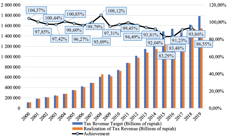
Figure 1. The development of tax revenue target, the realization of tax revenue, and achievement of tax revenue in Indonesia, 2000–2019.
Source: Author’s preparation (2021)
b. Development of macroeconomic variables: gross domestic product, inflation rate, interest rate (BI rate) and exchange rate (exchange rate of rupiah against US Dollar) in Indonesia
Government’s involvement in managing the economy is covered by public finance, and changes to either government expenditure or revenue (through taxes) are necessary to produce the desired effects (Hadi & Hashim, 2021). GDP demonstrates how much additional public revenue economic activity will produce over a specific time frame. The Indonesian economy grows annually. Specifically, in 2000, GDP amounted to 1.39 trillion rupiahs. Based on that time, GDP has continued to increase until 2019. In 2019, Indonesia’s GDP is 15,834 trillion rupiahs, with an average annual growth of 13.79%. During the 2000–2019 period, the highest GDP growth was seen in 2008, with a 25.25% increase from 2007 despite the 2007–2008 global financial crisis. The 2015–2019 period witnessed the lowest GDP growth, which was only below 10%, whereas in the previous years, namely 2000–2014, GDP growth was always above 10%. In 2019, Indonesia’s GDP growth only increased 6.71% from 2018, which represented the lowest GDP growth during the 2000–2019 period (Table 2).
The propensity for prices to grow consistently and widely is known as inflation. During the 2000–2019 period, the inflation rate in Indonesia tended to fluctuate, with an average of 6.76% per year (Table 2). From 2000 to 2008, the inflation rate in Indonesia was quite volatile, with an average of 9.42%. During the period 2000–2008, the lowest inflation rate occurred in 2003 at 5.06%, and the highest in 2005 at 17.11%. In the following period, namely 2009–2019, the inflation rate in Indonesia was relatively low (mild) and stable, with an average of 4.58%. In the period 2009–2019, the highest inflation rate occurred in 2013 at 8.38% and the lowest was seen in 2019, amounting to 2.72%.
Table 2. The Development of Indonesia’s GDP by Expenditure, Inflation, BI Rate, and Bank Indonesia Middle Exchange Rate (Rupiah against US Dollar), 2000–2019.
|
Year |
GDP (Billions of rupiah) |
GDP Growth |
Inflation |
BI rate |
Exchange Rate |
|
2000 |
1,389,770 |
– |
9.35% |
14.53% |
9,595 |
|
2001 |
1,646,322 |
18.46% |
12.55% |
17.62% |
10,400 |
|
2002 |
1,821,833 |
10.66% |
10.03% |
12.93% |
8,940 |
|
2003 |
2,013,675 |
10.53% |
5.06% |
8.31% |
8,465 |
|
2004 |
2,295,826 |
14.01% |
6.40% |
5.92% |
9,290 |
|
2005 |
2,774,281 |
20.84% |
17.11% |
12.75% |
9,830 |
|
2006 |
3,339,217 |
20.36% |
6.60% |
9.75% |
9,020 |
|
2007 |
3,950,893 |
18.32% |
6.59% |
8.00% |
9,419 |
|
2008 |
4,948,688 |
25.25% |
11.06% |
9.25% |
10,950 |
|
2009 |
5,605,203 |
13.27% |
2.78% |
6.50% |
9,400 |
|
2010 |
6,864,133 |
22.46% |
6.96% |
6.50% |
8,991 |
|
2011 |
7,831,726 |
14.10% |
3.79% |
6.50% |
9,068 |
|
2012 |
8,615,705 |
10.01% |
4.30% |
5.75% |
9,670 |
|
2013 |
9,546,134 |
10.80% |
8.38% |
7.50% |
12,189 |
|
2014 |
10,569,705 |
10.72% |
8.36% |
7.75% |
12,440 |
|
2015 |
11,526,333 |
9.05% |
3.35% |
7.50% |
13,795 |
|
2016 |
12,401,729 |
7.59% |
3.02% |
4.75% |
13,436 |
|
2017 |
13,589,826 |
9.58% |
3.61% |
4.25% |
13,548 |
|
2018 |
14,838,312 |
9.19% |
3.13% |
6.00% |
14,481 |
|
2019 |
15,833,943 |
6.71% |
2.72% |
5.00% |
13,901 |
|
Average |
7,070,163 |
13.79% |
6.76% |
8.35% |
10,841 |
Source: Author’s preparation (2021)
One of the financial tools chosen by Bank Indonesia to preserve economic stability is the BI rate. If future inflation is anticipated to surpass the predetermined objective, Bank Indonesia will typically increase the BI rate taking into account elements in the economy. In contrast, if future inflation is projected to be less than the predetermined objective, Bank Indonesia will reduce the BI rate (Bank Indonesia, n.d.). The BI rate during the 2000–2019 period averaged 8.35% per year (Table 2). From 2000 to 2008, the BI rate tended to fluctuate, with an average of 11.01% per year. The lowest BI rate was in 2004 at 5.92%, and the highest was in 2001 at 17.62%. In the following period, namely 2009-2019, the BI rate was relatively low and stable with an average of 6.18%. In the period 2009–2019, the highest BI rate occurred in 2014 at 7.75% and the lowest was in 2017 at 4.25%.
The exchange rate is needed to convert revenue and expenditure items in the Draft State Budget and the State Budget, whose original value is in US dollars. The development of the exchange rate in Indonesia during the 2000–2019 period tended to depreciate and fluctuate, with an average of 10,841 rupiahs per US dollar (Table 2). As a result of Indonesia’s monetary crisis, which started in 1997 and led to social unrest and political upheaval symbolized by the fall of the New Order regime, the exchange rate started to decline, falling by almost 100%. In the period 2000 to 2012, the exchange rate fluctuated with an average of 9,464 rupiahs per US dollar. In the last seven years, namely 2013–2019, the exchange rate has continued to depreciate every year and is above 10,000 rupiahs per US dollar. The average exchange rate during the 2013–2019 period was IDR 13,399 per US dollar. In 2019, the exchange rate was recorded at 13,901 rupiahs per US dollar.
Graph of development of macroeconomic variables: gross domestic product (GDP) (Figure 2); inflation rate, interest rate (BI rate), and exchange rate (rupiah exchange rate against US dollar) in Indonesia during the 2000–2019 period (Figure 3).
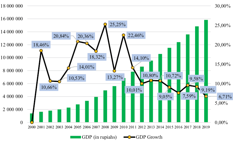
Figure 2. The development of gross domestic product (GDP) in Indonesia, 2000–2019.
Source: Author’s preparation (2021)
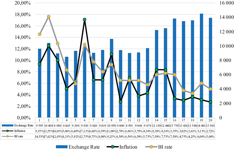
Figure 3. The development of inflation rate, interest rate (BI rate), and exchange rate (rupiah exchange rate against US dollar) in Indonesia, 2000–2019.
Source: Author’s preparation (2021)
3.1.2. Quantitative Analysis
This study used the Augmented Dickey–Fuller (ADF) test to assess stationarity. Table 3 displays the outcomes of the unit roots test performed using the ADF technique.
Table 3. Unit Root Test Values with the ADF Test Method to Assess the Stationarity of Macroeconomic Variables.
|
Variable |
ADF Test Value |
Mackinnon Critical Value 5% |
Probability |
Decision |
|
LTAX |
−2.944404 |
−3.040391 |
0.0598 |
Not Stationary |
|
LGDP |
−2.723112 |
−3.029970 |
0.0886 |
Not Stationary |
|
LNTR |
−0.736190 |
−3.029970 |
0.8142 |
Not Stationary |
|
INF |
−3.257379 |
−3.029970 |
0.0321 |
Stationary |
|
BIR |
−0.554854 |
−3.081002 |
0.8536 |
Not Stationary |
Source: Author’s preparation (2021)
It is required to test the degree of integration because not all variables are stationary at the unit root according to the ADF test with a 5-percent Mackinnon critical value. Table 4 displays the outcomes of the degree of integration test using the ADF method on the first differentiation.
Table 4. Test Value of the Degree of Integration with the ADF Test Method in the First Difference to Assess the Stationarity of Macroeconomic Variables.
|
Variable |
ADF Test Value |
Mackinnon Critical Value 5% |
Probability |
Decision |
|
LTAX |
−5.492166 |
−3.040391 |
0.0004 |
Stationary |
|
LGDP |
−0.913025 |
−3.052169 |
0.7582 |
Not Stationary |
|
LNTR |
−4.298303 |
−3.040391 |
0.0041 |
Stationary |
|
INF |
−6.543999 |
−3.052169 |
0.0001 |
Stationary |
|
BIR |
−4.569856 |
−3.052169 |
0.0026 |
Stationary |
Source: Author’s preparation (2021)
It is important to test the degree of integration on the second differentiation since, according to the ADF test on the first differentiation, not all variables are stationary at the Mackinnon critical value of 5%. Table 5 displays the outcomes of the degree of integration test using the ADF method on the second differentiation.
Table 5. Test Value of the Degree of Integration with the ADF Test Method in the Second Difference to Assess the Stationarity of Macroeconomic Variables.
|
Variable |
ADF Test Value |
Mackinnon Critical Value 5% |
Probability |
Decision |
|
LTAX |
−5.831463 |
−3.065585 |
0.0003 |
Stationary |
|
LGDP |
−6.833292 |
−3.052169 |
0.0000 |
Stationary |
|
LNTR |
−6.279194 |
−3.052169 |
0.0001 |
Stationary |
|
INF |
−7.930813 |
−3.065585 |
0.0000 |
Stationary |
|
BIR |
−5.586079 |
−3.065585 |
0.0004 |
Stationary |
Source: Author’s preparation (2021)
Based on the ADF test on the differentiation of the two variables, all variables are stationary at the Mackinnon critical value of 5% and are ready for use in ECM analysis.
To calculate the ADF value, a cointegration regression equation is conducted with the ordinary least squares method. The results of the regression equation above can be seen in Table 6.
Table 6. The Cointegration Regression Equation Test of Macroeconomic Variables Effect in Long Run Tax Revenue using Ordinary Least Squares Estimator
|
Variable |
Coefficient |
t-statistic |
Probability |
Adjusted R² |
|
C |
0.060642 |
0.047831ᵈ |
0.9625 |
0.985866 |
|
LGDP |
0.989811 |
13.94075* |
0.0000 |
|
|
INF |
2.073099 |
2.298586** |
0.0363 |
|
|
BIR |
−2.164240 |
−1.542970ᵈ |
0.1437 |
|
|
LNTR |
−0.222131 |
−1.045768ᵈ |
0.3122 |
Source: Author’s preparation (2021)
Note:
* significant at 1% confidence level
** significant at 5% confidence level
*** significant at 10% confidence level
d not significant
From the regression equation, the residual value is obtained. Furthermore, this residual value will be tested using the ADF test to determine whether the residual value is stationary. The ADF test results can be seen in Table 7 below.
Table 7. Value of Cointegration Test with the ADF Method at Long Term Stationary Test
|
Variable |
ADF Test Value |
Mackinnon Critical Value 5% |
Probability |
Decision |
|
Residual |
−5.977329 |
−3.029970 |
0.0001 |
Stationary |
Source: Author’s preparation (2021)
From the results of the cointegration test using the ADF method in Table 7, it can be seen that the residual absolute value of ADF is −5.977329 > 5% critical value, which is −3.029970, thus, the residual has been stationary and there is cointegration between the variables.
According to the results of the cointegration test, data from a stationary study have a long-term link between the independent and dependent variables. The residuals from the cointegrated equation or the long-run equation can then be used to create an ECM model. To determine the short-term equation, the ECM test is run. The formation of the ECM model is intended to determine which changes in the variables between GDP, INF, BIR and NTR have a significant effect (in the short term) on TAX. Based on the dynamic model of the ECM approach, the regression estimation results are as shown in Table 8.
Table 8. Equation Approach Estimation of Macroeconomic Variables Effect in Short Run Tax Revenue Using the ECM Test
|
Variable |
Coefficient |
t-statistic |
Probability |
Adjusted R² |
|
C |
−0.068891 |
−1.755514*** |
0.1027 |
0.792880 |
|
D(LGDP) |
1.529412 |
5.515026* |
0.0001 |
|
|
D(INF) |
1.076803 |
2.515695** |
0.0258 |
|
|
D(BIR) |
−2.310360 |
−2.699231** |
0.0182 |
|
|
D(LNTR) |
0.204817 |
1.250076ᵈ |
0.2333 |
|
|
ECT(−1) |
−0.978086 |
−5.435084* |
0.0001 |
Source: Author’s preparation (2021)
The amount of cointegration coefficient that functions as an adjustment element (speed of adjustment), namely ECT, is negative at -0.978086 with a probability of 0.0001 < than the value α = 5% (0.05) with a confidence level of 95%. Therefore, this ECM model can be said to be valid.
Long-Run Equation
LTAX = 0.060642 + 0.989811 LGDP + 2.073099 INF –2.164240 BIR – 0.222131LNTR (3)
Short-Term Equation:
DLTAX = –0.068891 + 1.529412 DLGDP + 1.076803 DINF – 2.310360 DBIR + 0.204817 DLNTR – 0.978086 (ECT) – 1 (4)
From the ECM equation model, it can be seen that the cointegration coefficient that functions as an adjustment element (speed of adjustment), namely ECT, is negative at −0.978086 with a significant probability at α = 5% (0.05), which is equal to 0.0001. Therefore, this ECM testing model can be said to be valid. The ECT coefficient value of −0.978086 indicates that short-term balance fluctuations will be corrected towards long-term equilibrium. In the first year, 97.81% of the adjustment process occurs and 2.19% of the adjustment process manifests in the following years.
The mutual signification test (F-statistic test) showed that the results of OLS processing for the long term calculated F value (F-statistic) is 332.3100 with a probability of 0.000000 < the value of α = 5% (0.05), with a 95% confidence level. The results of data processing for the short term using ECM analysis produce a calculated F value of 14.78123, with a significant F-statistical probability, which is equal to 0.000057 < than the value of α = 5%. Thus it can be concluded that the independent variables (GDP, inflation, BI rate and exchange rate) together have a significant effect on the dependent variable (tax revenue).
The coefficient of determination test based on the results of processing the OLS model data for the long term obtained an adjusted R² of 0.985866, while the results of data processing for the ECM model obtained an adjusted R² value of 0.792880, meaning that the influence of the independent variables GDP, inflation, BI rate, and the exchange rate affects the dependent variable of revenue tax in Indonesia is 79.29%. The remaining 20.71% is influenced by variables outside the model.
3.2. Discussion
Tax revenue is the most significant source of state revenues influencing the entire economic system and the country’s development. The future direction and amount of tax revenue should be well determined to prepare the State Budget and set the projection of economic activity growth of a nation. Several macroeconomic indicators’ performance have been studied to have relationship to the tax revenue. In this study, the effect of four macroeconomic variables, i.e. GDP, inflation, interest rates, and exchange rates, to the Indonesia’s tax revenue in long- and short-term are analyzed using ECM. The results showed that each variable has different effect on the tax revenue.
3.2.1. Effect of GDP
Based on research conducted in several countries, macroeconomic imbalances and levels of economic activity are the main factors or drivers of tax elasticity or tax revenue (Muibi and Sinbo, 2013). Government tax revenue depends not only on changes in tax policy but also on many other macroeconomic factors. Though there are changes in tax policy, several macroeconomic factors are able to influence tax collection (Neog and Gaur, 2020). The quantitative analysis’s findings show that the GDP variable’s positive and considerable impact on tax revenue in the long- and short-term estimation (ECM) is represented by the results. A number of other studies connect the pattern of relationships between GDP and tax revenue and come to the same conclusion: GDP has a positive and considerable impact on tax revenue (Ariwayo, 2018; Babatunde et al., 2017; Dahal, 2020; Handoko et al., 2014; Muibi and Sinbo, 2013; Zhang and Cui, 2008).
This long- and short-term positive significant effect is also illustrated from the results of the descriptive analysis. During the 2000–2019 period, 2008 was the year with the highest GDP growth, namely an increase of 25.25% from 2007. This is in line with the realization of tax revenues in 2008, which reached 108.12% of the target set and was also the highest percentage of achievement during the 2000–2019 period. The 2015–2019 period witnessed the lowest GDP growth, which was below 10%, whereas in previous years, namely 2000–2014, GDP growth was always above 10%. The lean period aligns with the realization of tax revenue in the last five years, namely 2015–2019, which saw the largest tax revenue shortfalls, with an average percentage of tax revenue target achievement of only 87.68% per year.
3.2.2. Effect of Inflation (INF)
Inflation will reduce the purchasing power of money that has been obtained by the public. Inflation causes an increase in production costs and a decrease in sales, which results in a decrease in producer income, which is the basis for taxation. The existence of inflation will also lead to a fall in economic activity, which in turn results in less money coming in as taxes. The outcomes of the quantitative research demonstrated a strong positive long- and short-term association between INF and TAX. Theoretically, the link between INF and TAX should be negative, but this result contradicts that. Numerous research examining the relationship between the pattern of the inflation rate and tax revenue have also discovered results that defy theory, namely, that inflation has a favorable and considerable impact on tax income (Ariwayo, 2018; Renata and Hidayat, 2016; Zaroomi et al., 2020)
This long- and short-term positive significant effect is also illustrated from the results of the descriptive analysis. The inflation rate in Indonesia during the period 2000–2008 was quite high and fluctuating, with an average of 9.42% per year. The high rate of inflation during the 2000–2008 period had no negative effect on tax revenue. The average tax revenue realization during the 2000–2008 period actually reached 100.41% of the predetermined target. The inflation rate in Indonesia for the last five years, namely 2015–2019, tends to be low and stable, with an average of 3.17% per year. This condition is different from the previous two years, namely 2013–2014, where the inflation rate was above 8%. In fact, the low and stable inflation rate during the 2015–2019 period did not affect the realization of tax revenue. In the last five years, tax revenue has experienced the largest shortfall, with an average percentage of tax revenue achievement of only 87.68% per year.
According to the study’s findings, tax revenue is positively and significantly impacted by inflation. This is so because rising inflation rates lead to higher selling prices, which raise tax receipts. The positive effect of inflation on tax revenue might also be assumed when inflation is low and can be controlled by the government; however, companies and society do not respond to low inflation. Therefore, even with a decrease in the rate of inflation, companies tend not to increase their investment activities. The same occurs with economic transactions carried out by the public, which in the end do not lead to an increase in tax revenue. In fact, lower inflation reduces tax revenues due to low selling prices.
3.2.3. Effect of the Bank Indonesia Interest Rate (BIR)
An increase in BI interest rates (BIR) results in an increase in interest rates at commercial banks, which will make people more likely to save their money in banks compared to investing in the real sector. Consequently, employment decreases, which results in a reduction in tax revenue. A rise in interest rates will also reduce public consumption patterns, and a decrease in public consumption results in lowered tax revenues. From the results of the quantitative analysis, BIR has a negative insignificant effect in the long run on TAX. This finding is also illustrated by the results of the descriptive analysis in which BIR fluctuated from 2000 to 2008, with an average of 11.01% per year. BIR fluctuations during the 2000–2008 period did not really affect TAX. During the 2000–2008 period, the average TAX reached 100.41% per year from the target set by the government. The low and stable BIR during the 2009–2019 period also had no effect on TAX. In the 2009–2019 period, TAX always experienced a shortfall every year with a percentage of achievement of 92.05% annually. In the long term, BIR has no effect on TAX because during the research period (2000–2019) the BIR set by Bank Indonesia was still accommodative to the Indonesian economy. During the 2000–2019 period, the average BIR was 8.35% per year, with an accommodative BIR interest rate, which did not significantly affect economic transactions conducted by investors and the public.
In line with theory, the results of the quantitative analysis of BIR have a significant negative effect on TAX in the short term. This negative relationship between BIR and TAX is also illustrated by the results of the descriptive analysis. The high BIR rate in 2001 was 17.62%, which during the 2000–2019 period was the highest BIR rate. The high BIR in 2001 received a negative response, with the percentage of TAX achievement in 2001 of 100.44% of the set target, down 3.09% compared to the previous year, whereas in 2000, the percentage of TAX reached 104.37% of the set target. This condition was also reflected in 2005, where BIR increased by 6.83 points compared to the previous year, namely to 12.75%, whereas in 2004 BIR was only 5.92%. The increase in BIR received a negative response with a TAX shortfall in 2005. The percentage of TAX achievement fell compared to the previous year, which was 98.60% of the set target, a decrease of 2.25% compared to the previous year. This result compares with 2004, where the percentage of TAX reached 100, which is 85% of the target set. The significant negative result of the BIR on tax revenue in the short term is thought to be due to the direct response of the BIR rate increase by banks by increasing the credit interest rate. The decision of the banking sector to raise credit interest rates resulted in companies reducing their investment activities, and the public also reduced economic transactions, which in turn reduced tax revenues.
3.2.4. Effect of Exchange Rates (NTR)
Due to the tendency of investors to exercise caution when making investments, the exchange rate is one of the indications that influence activity in the stock market and money market. The economy and the stock market are negatively impacted by the drop in the rupiah’s exchange rate versus other currencies, particularly the US dollar. Following is the method by which the exchange rate has a negative impact on tax collection. The cost of producing products and services rises as a result of an increase in the exchange rate (weakening versus the dollar), which is then passed on to the consumer in the final selling price. Higher prices weaken consumer purchasing power, which ultimately decreases tax revenue. In sum, currency depreciation results in a general increase in domestic price levels, which results in a decrease in consumer purchasing power (Wilya, 2015). In the end, tax revenues are reduced.
The NTR variable in the long-term estimation demonstrates that NTR has a negative negligible connection with TAX based on the findings of the quantitative study. The short-term estimation (ECM) shows that the NTR has a positive insignificant relationship with TAX. That is, TAX is not affected by changes in NTR. According to theory, there is a relationship between NTR and TAX that influences how much the rupiah appreciates (NTR weakens/strengthens), and as a result, TAX is expected to rise. This finding contradicts that idea. Divergent outcomes from the idea have been observed in several research that link the pattern of the relationship between the exchange rate (rupiah exchange rate) and tax income. For example, a study conducted by Mispiyanti & Kristanti (2018) showed that the impact of the exchange rate on tax receipts is negative and negligible. In the meanwhile, studies by Sumidartini (2018), a different set of findings, namely that the impact of the exchange rate on tax collection is both favorable and considerable.
The nonsignificant negative relationship between NTR and TAX in the long term can be seen from the results of the descriptive analysis, where the development of Indonesia’s NTR during the 2000–2019 period tended to fluctuate and depreciate. The average NTR during the 2000–2019 period was IDR 10,841 per US dollar. TAX during the period 2000–2019 averaged 765 trillion rupiahs per year with the percentage of achievement against the target set by the government of 95.81% per year. TAX development during 2000–2019 tended to move below the target set or experienced a shortfall.
The insignificant positive relationship between NTR and TAX in the short term is illustrated by TAX in 2008, which reached 108.12% of the predetermined target, which is the highest percentage of achievement during the 2000–2019 period. This is in line with the NTR in 2008, where the rupiah depreciated by 1,531 points compared to 2007, to 10,950 rupiahs per US dollar. This compares with previous periods, namely 2002–2008, where the movement of the rupiah against the US dollar was still below 10,000 rupiahs per US dollar. Depreciation (the rupiah exchange rate up or down against the US dollar) in 2008 was followed by an increase in the realization of tax revenues in 2008.
3.2.5. The relationship and influence between macroeconomic variables and tax revenues
Macroeconomics is observed to have a very significant relationship and influence on tax revenues, this is indicated by the adjusted R² value of 0.792880 from the results of the ECM analysis. It means that the influence of macroeconomic variables used in this study is very significant on taxes income in Indonesia with a percentage of 79.29%, while the remaining 20.71% is influenced by variables outside the external model. The previous studies in other countries found the same evidence, that if the government wants to increase tax revenues, then the important thing that the government must pay attention to is guaranteeing macroeconomic conditions in the country. In China, the coordination between macroeconomics and tax revenues is needed, and it should be the basic rule when making tax policy (Zhenyu & Huqin, 2009). The same condition was found in Nigeria, in which the macroeconomic instability and the level of economic activity are the main drivers of tax collection (Muibi and Sinbo, 2013). A study conducted by Babatunde et al. (2017) in Africa in determining the taxation revenue and economic growth in Africa, showed that in developing a comprehensive tax structure or model, the government must pay attention to the country’s macroeconomic conditions, so that the applied tax structure can grow, maintain and maintain its tax economic base so as to encourage economic performance. Mirović et al. (2019), who examined the modelling of tax influence in Spain, stated that the form of tax is closely related to the macroeconomic framework. These statements are strengthened by a research conducted to determine the factors influencing tax revenues in India; it showed an evidence that several macroeconomic variables are determinants affecting the performance of tax revenues (Neog and Gaur, 2020).
The results of the current study, as well as empirical evidence in several other countries, show that the amount of future tax revenue will be largely determined by the influence of macroeconomic variables. Thus, the government must pay attention to and maintain the stability of macroeconomic variables, so that the target or increase in tax revenue can be realized.
4. Conclusion and recommendation
This study provides input for the government in implementing fiscal policy, concluding that the determination of the tax revenue target amount must better reflect indicators of ongoing macroeconomic conditions to be more realistic in accordance with economic developments. The setting of unrealistic tax revenue targets will have an impact on the government’s failure to carry out its budgetary functions.
Related to its strategic role in the country’s economy, taxes experience risk in the form of realized tax revenues outside the targets set by the government or known as a shortfall. The trend of tax shortfall in Indonesia began in 2002 and continues to occur and has increased yearly. As stated in theory and also proven from research results, the influence of macroeconomic variables, which consist of gross domestic product (GDP), inflation (INF), BI Rate (BIR), and exchange rate (rupiah exchange rate against the US dollar NTR), on tax revenue, especially that of GDP has a very dominant influence on tax revenue both in the long and short term.
The response of tax revenue to economic development must be even greater because the larger the response of tax revenue to the increase and development of macroeconomic indicators, the greater the potential for increased tax revenue. The government must also maintain the stability of macroeconomic variables. As demonstrated in this study, there is a strong influence of macroeconomic variables on tax revenues in both the long and short term.
Fiscal policy is essential for a country’s economy, especially when the economy is experiencing a slowdown. Government spending and taxation are forms of fiscal policy that stimulate a country’s economy. Fiscal policy in the form of tax revenue will increase revenue in a country. The greater state revenue will increase the amount of state spending, and with the increase in state spending, the GDP will also increase. In fact, GDP will increase more than public spending if government spending is allocated to the domestic sector; this can result in a multiplier effect, making the country’s economy grow and develop. The development of the economy will increase state revenues, especially tax revenues.
It is concluded that the changes in the future tax revenues are largely determined by the stability of macroeconomic variables. Therefore, the policymakers or the government should implement policies that can maintain the stability of macroeconomic variables so that an increase in the scope of tax revenue can be realized. Some of the most basic policies that the government or policymakers can implement are to ensure that the government has good legitimacy, accountability, and responsiveness to developing economic, social, and political conditions within and outside the country.
The findings in this study could become empirical knowledge and broaden insights regarding taxation and the economy in Indonesia, which of course, can also be applied and developed by other countries, especially countries whose state financial conditions are the same as Indonesia. The mechanisms regarding steps or policies that must be taken by the government to maintain the stability of macroeconomic variables that affect tax revenue is recommended for further research.
5. Declarations
The contents of the paper have been reviewed and approved by each co-author, and there are no competing financial interests to disclose. We attest that the submission is unique and is not already being considered by another scientific journal.
References
Adam, A., Kammas, P., & Lapatinas, A. (2015). Income inequality and the tax structure: evidence from developed and developing countries. Journal of Comparative Economics, 43(1), 138–154. https://doi.org/10.1016/j.jce.2014.05.006
Ariwayo, O. R. (2018). A study on the determinants of tax revenues in Africa. Lisbon School of Economics and Management.
Babatunde, O. A., Ibukun, A. O., & Oyeyemi, O. G. (2017). Taxation revenue and economic growth in Africa. Journal of Accounting and Taxation, 9(2), 11–22. https://doi.org/10.5897/jat2016.0236
Bank Indonesia. (n.d.). Tujuan kebijakan moneter. Retrieved April 6, 2021, from https://www.bi.go.id/id/fungsi-utama/moneter/default.aspx [Indonesian]
Dahal, A. K. (2020). Tax-to-GDP ratio and the relation of tax revenue with GDP: Nepalese perspective. Researcher: A Research Journal of Culture and Society, 4(1), 80–96. https://doi.org/10.3126/researcher.v4i1.33813
Engle, R. F., & Granger, C. W. J. (1987). Co-integration and error correction: representation, estimation, and testing. Journal of The Economectric Society, 55(2), 251–276. https://doi.org/10.2307/1913236
Fjeldstad, O.-H. (2014). Tax and development: donor support to strengthen tax systems in developing countries. Public Administration and Development, 34, 182–193. https://doi.org/10.1002/pad.1676
Granger, C. W. J. (1980). Long memory relationships and the aggregation of dynamic models. Journal of Econometrics, 14(2), 227–238. https://doi.org/10.1016/0304-4076(80)90092-5
Granger, C. W. J., & Weiss, A. A. (1983). Time series analysis of error-correction models. In Studies in Econometrics, Time Series, and Multivariate Statistics. Elsevier. https://doi.org/10.1016/b978-0-12-398750-1.50018-8
Hadi, A. R. A., & Hashim, M. H. (2021). Malaysia government revenue and public debt - 1970 through 2019. Psychology and Education, 58(2), 2080–2088. https://doi.org/10.17762/pae.v58i2.2374
Handoko, I., Aimon, H., & Sofyan, E. (2014). Analisis faktor-faktor yang mempengaruhi perekonomian dan penerimaan pajak di Indonesia. In Jurnal Kajian Ekonomi, Juli (Vol. 3, Issue 5) [Indonesian]
Harahap, M., Sinaga, B. M., Manurung, A. H., & Maulana, T. N. A. (2018). Impact of Policies and macroeconomic variables on tax revenue and effective tax rate of infrastructure, utility, and transportation sector companies listed in Indonesia stock exchange. International Journal of Economics and Financial Issues, 8(3), 95–104. http:www.econjournals.com
Kalaš, B., Mirović, V., & Milenković, N. (2018). The relationship between taxes and economic growth: evidence from Serbia and Croatia. The European Journal of Applied Economics, 15(2), 17–28. https://doi.org/10.5937/EJAE15-18056
Kementerian Keuangan. (2020). Nota Keuangan beserta Anggaran Pendapatan dan Belanja Negara Tahun Anggaran 2020 (II, Issue Defisit dan Pembiayaan Anggaran) [Indonesian]
Kementerian Keuangan Republik Indonesia, Direktorat Jenderal Anggaran, D. P. A. (2014). Dasar-dasar praktek penyusunan APBN di Indonesia (Purwiyanto & K. W. D. Nugraha (eds.); II). https://doi.org/10.1017/CBO9781107415324.004 [Indonesian]
Kim, J., Wang, M., Park, D., & Petalcorin, C. C. (2021). Fiscal policy and economic growth: some evidence from China. Review of World Economics, 157(3), 555–582. https://doi.org/10.1007/s10290-021-00414-5
Milasi, S., & Waldmann, R. J. (2018). Top marginal taxation and economic growth. Applied Economics, 50(19), 2156–2170. https://doi.org/10.1080/00036846.2017.1392001
Mirović, V., Kalaš, B., & Andrašić, J. (2019). The modelling of tax influence on macroeconomic framework in Spain. Economic Analysis, 52(2), 128–136. https://doi.org/10.28934/ea.19.52.2.pp128-136
Mispiyanti, M., & Kristanti, I. N. (2018). Analisis pengaruh PDRB, inflasi, nilai kurs, dan tenaga kerja terhadap penerimaan pajak pada Kabupaten Cilacap, Banyumas, Purbalingga, Kebumen dan Purworejo. Jurnal Ilmiah Akuntansi Dan Keuangan, 7(1), 23–37. https://doi.org/10.32639/jiak.v7i1.159 [Indonesian]
Muibi, S. O., & Sinbo, O. O. (2013). Macroeconomic determinants of tax revenue in Nigeria (1970-2011). World Applied Sciences Journal, 28(1), 27–35. https://doi.org/10.5829/idosi.wasj.2013.28.01.1189
Neog, Y., & Gaur, A. K. (2020). Macro-economic determinants of tax revenue in India: an application of dynamic simultaneous equation model. International Journal of Economic Policy in Emerging Economies, 13(1), 13–35. https://doi.org/10.1504/IJEPEE.2020.106682
Ozili, P. K. (2020). Tax evasion and financial instability. Journal of Financial Crime, 27(2), 531–539. https://doi.org/10.1108/JFC-04-2019-0051
Undang-Undang Republik Indonesia Nomor 17 Tahun 2003 tentang Keuangan Negara, Kementerian Sekretariat Negara 1 (2003) [Indonesian]
Renata, A. H., Hidayat, K., & Kaniskha, B. (2016). Pengaruh inflasi, nilai tukar rupiah dan jumlah pengusaha kena pajak terhadap penerimaan pajak pertambahan nilai (studi pada Kantor Wilayah DJP Jawa Timur I). Jurnal Perpajakan (JEJAK), 9(1), 1–9. [Indonesian]
Sawhney, U. (2018). An analysis of fiscal policy in an emerging economy: innovative and sustainable fiscal rules in India. Millennial Asia, 9(3), 295–317. https://doi.org/10.1177/0976399618805629
Skarzauskas, S. (2021). Evaluating impact of tax Burden on state financial stability: empirical research of EU countries. Theoretical Economics Letters, 11(06), 1122–1139. https://doi.org/10.4236/tel.2021.116071
Stoilova, D. (2017). Sistema fiscal y el crecimiento económico: evidencia de la Unión Europea. Contaduria y Administracion, 62(3), 1041–1057. https://doi.org/10.1016/j.cya.2017.04.006
Sumidartini, A. N. (2018). Pengaruh nilai tukar rupiah serta tingkat suku Bunga terhadap penerimaan pajak pada Direktorat Jenderal Pajak. Transparansi Jurnal Ilmiah Ilmu Administrasi, 9(1), 53–68. https://doi.org/10.31334/trans.v9i1.85 [Indonesian]
Wilya. R, S., Putro, T. S., & Mayes, A. (2015). Pengaruh produk domestik bruto, inflasi dan capital account terhadap nilai tukar rupiah atas dollar Amerika Serikat periode tahun 2001-2014. Jom FEKON, 2(2), 1–13 [Indonesian]
Yossinomita. (2022). Tax policy in limiting the consumption of luxury goods. Review of Economics and Finance, 20(1), 165–171. https://doi.org/10.55365/1923.x2022.20.19
Zaroomi, H. K., Samimi, A. J., & Potanlar, S. K. (2020). The impact of inflation targeting on direct taxes in selected countries: a propensity score matching (PSM) approach. International Journal of Economics and Politics, 1(2), 133–151. https://doi.org/10.29252/jep.1.2.133
Zhang, M. Y., & Cui, J. C. (2008). A cointegration analysis of the relationships among tax revenue and macroeconomic factors in China. The 7th International Symposium on Operation Research and Its Application (ISORA’08), 260–265.
Zheng, L., & Severe, S. (2016). Teaching the macroeconomic effects of tax cuts with a quasi-experiment. Economic Analysis and Policy, 51, 55–65. https://doi.org/10.1016/j.eap.2016.06.001
Zhenyu, L., & Huqin, Y. (2009). Analysis of coordination between tax revenue and macroeconomics in China. Proceedings of 2007 International Conference on Management Science and Engineering, ICMSE’07 (14th), August, 1789–1795. https://doi.org/10.2139/ssrn.1445184